AI Unplugged 21: TPI LLM, Differential Transformer, ARIA, Ministral 3B and 8B

Insights over information.

Table of Contents:

1. TPI LLM: Serving 70B LLMs on edge devices

2. Differential Transformer

3. Aria : An Open Multimodal Native Mixture-of-Experts Model

4. Ministraux: MiniStral 3B and 8B.

Previous Edition

TPI LLM: Serving 70B LLMs on edge devices

TLDR: 
    Serving LLMs, that too the larger ones on edge devices is a challenge. Tensor Parallelism comes out better than Pipeline parallelism for such cases. Also loading weights asynchronously while some other computation happens or helps relieve memory size limits. Also to ensure privacy, the master device has to take care of embedding and un-embedding so that all the workers see is untraceable hidden states.

So you must be wondering how is it even possible? LLMs are memory hogs, even more than Google Chrome, how can they run on edge devices. Well you’re not entirely wrong there. An LLM as small as (isn’t that an oxymoron calling LLM small?) 7B params would need 16GB memory to run in 16 bit precision (bfloat16/float16). Well you might ask why not go to some lower quantisation like int8 or int4/float4 or even 2 bit quantisation? When talking about edge devices, mostly CPUs and maybe even older GPUs, they don’t natively have support for these fancy data types. So a lot of time would be lost in typecasting these to full precision (FP32) in the first place.

So what can we do then? Well when one doesn’t do the trick, bring in more. One machine is slow and low on resources but what about 4 together? How about 8? Sounds like a plan right (Apes together strong)? But even then we’d fall short by quite a big margin. Assuming an average 8GB RAM per device out of which say 4 GB is usable, we’d only have 32 GB for us to work with which can be enough for ~13-14B scale models. How does one dream of 70B models then? Well we don’t wanna have too many devices cuz getting such a network always available might not be feasible too. So let’s stick to 8 devices for now and try to work around the memory capacity constraints.

We’ve decided that we want to use multiple devices for inference. Now the question arises, how do you split the model up across devices? Well there are two popular approaches. Pipeline Parallelism and Tensor Parallelism. You can read more about those here. But in a nutshell, pipeline parallelism allocates each layer to a device and the result is shared across. This is like splitting the model depth wise. In Tensor Parallelism, each layer’s weights are split across devices. This is like splitting the model width wise. Here’s a pretty bad visual graphic of the same :)

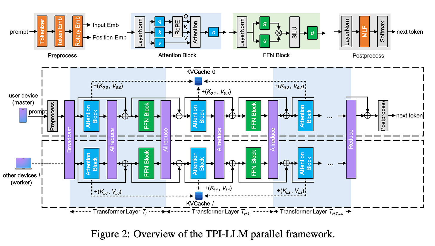
Among the said alternatives, what do you think is better for our case? Because we’re only worried about inference, at time step 1 when device 1 is processing layer 1, devices 2-n are idle in case of Pipeline parallelism (this changes for training when there’s are multiple batches of data). Hence Tensor Parallelism sounds like a more saner choice right? One thing to note in tensor parallelism is that because computation is split across devices, before passing through to the 2nd layer, all the devices’ output has to be gathered together and post processed (if needed).

For context before diving in, remember Flash Attention? The key idea there was in GPU regime, we’re bottlenecked by memory transfers. Flash attention comes up with custom kernels to reduce just that. Taking a leaf off of that book, first we need to identify what is our bottleneck here. There are three components. Memory transfer (from disk to memory), Computation (In memory) and Result sync ( across the network). Go ahead and think what would be probable bottleneck. With UFS 3.0 sequential reads reaching 2100Mbps, we’re pretty sure not bottlenecked by disk speeds. Network is a very plausible candidate as we’d be transferring activations (or parts of them) across the network across devices.

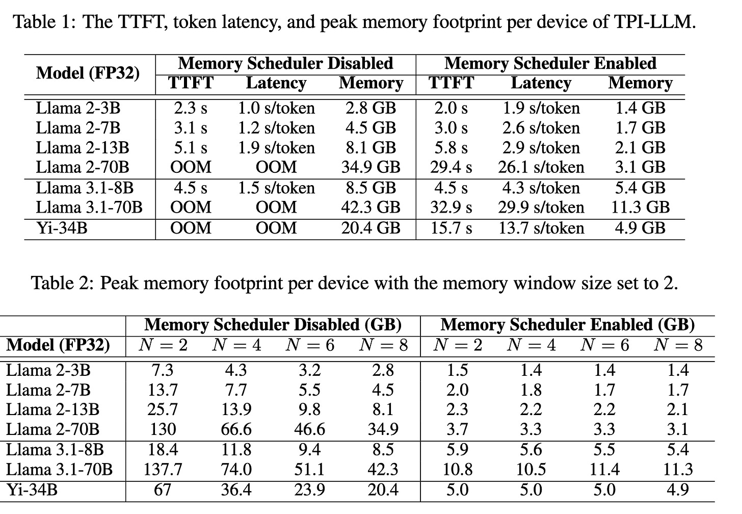
Here as we’re dealing with CPUs, we do have some time to deal with this memory capacity (in order of milliseconds but it is significant in terms of CPU clock cycles). If you understood what I’m hinting at, kudos. While we process layer 1, with the weights of layer 1 in memory, we can try to load up layer 2’s weights asynchronously. So at any stage you’d need memory to store the weights of a couple of layers (one can load more depending on the memory transfer vs compute vs network bandwidth, but you get the idea. For more info about what is suitable when, please read 3.2 Latency Analysis from the paper). Basically saying if weights loading takes less time than computation and network transfer of activations, we’re good with this. So theoretically speaking, lets say we have enough memory to load m layers. First we’d load layers 1-m, then when layer 1 is done, we drop if off back to disk and load layer m+1 weights at the same time. This fancy thing of loading weights in a sliding window fashion is named Memory Scheduling. Because we’re only loading what is needed, the peak memory usage wouldn’t grow as fast as the model size or the number of devices.

Now there’s one more problem. Again? Seriously? What is it now? Well privacy. You might not care about it but it matters. So how does one ensure privacy in such a setting? Well the only decodable pieces of information are the words themselves and the tokens. If we somehow hold them only on the requester’s device (aka master), we’re good. After all, the intermediate states aka activations (that too part of them) aren’t that sensitive and traceable anyway right. So to achieve this, the embedding and lm_head layers need to happen on the master device.

After every layer, we need to gather the information from all the nodes (All Reduce) and then collate that, broadcast it back to all the devices to let their compute happen. There are several ways to achieve this communication. One is a master and worker architecture where all the nodes talk to central node and it acts like the leader. Another is to exchange information to the neighbour in a circle and the information comes back to you few steps later. Both have their own advantages and disadvantages. The first is bottlenecked by how quick master can collate and return information. The second is limited by hop-time (time taken to send/receive information to/from neighbour). If the amount of data to be transferred is insignificant compared to link speed, like in our case where one needs to transfer hidden states (in the order of KBs), the master-worker approach, called as STAR (imagine the star graph where central node is connected to every other node via an edge) topology makes sense as it eliminates unnecessary hops.

So after all this trickery and mental gymnastics, how does the technique perform in comparison? Well here’s the results. If you can wait an average of 30s per token, great, you can very well run a 34B model at your home :) Taking us back to the days of old where small programs used to take seconds to execute.

Though not many would probably use this, its a cool work nonetheless. One has to understand mathematically where the bottleneck is to solve and optimise for it. One can extend the same to GPUs when the compute outperforms network. But for now GPUs are happy with NVLink. Note that the devices used for this work are in no way latest and greatest. So things are only gonna get better from here. Maybe some day one can truly do a distributed inference of LLMs across network and it won’t be bad :)

Differential Transformer

TLDR: 
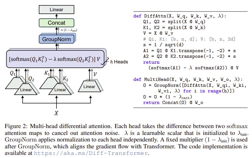
    The DIFF Transformer introduces a novel differential attention mechanism that enhances attention to relevant contexts by calculating scores from the difference of two softmax attention maps, effectively canceling noise.
     Experiments demonstrate Diff Transformer reaches same loss as Transformers in 38% fewer params or using 36% less training tokens. There's <10% hit to forward-backward pass performance. Turns out the outlier logits and activations are of lesser magnitude helping with Quantisation. There are improvements observed in in context and long context tasks.

In the ever-evolving landscape of Transformer models, a new contender has emerged: the Differential Transformer (Diff Transformer). This innovative model is designed to tackle the challenges faced by large language models (LLMs) in processing information efficiently. As we know, the classic Transformer, particularly its decoder-only variant, has dominated the LLM scene, largely due to its attention mechanism. This mechanism, relying on the softmax function, assigns importance to various tokens in a sequence. However, research reveals a common pitfall: standard Transformers struggle to pinpoint critical information when sifting through a sea of documents (this is why benchmarks like needle in a haystack and RULER are important). Instead of zeroing in on relevant details, they often succumb to what we call "attention noise," where irrelevant information distracts the model, hindering its ability to spotlight the right answer.

This paper introduces Diff Transformer, a solution designed to combat this attention noise. At the heart of this model lies a groundbreaking "differential attention mechanism." Each layer of the Diff Transformer is equipped with two main components: differential attention and a feed-forward network. The star of the show is the differential attention module, which replaces the traditional softmax-based attention mechanism. Instead of relying on a single softmax operation, this model employs two softmax functions and computes their difference. This clever design filters out the noise in attention scores, leading to sharper, more accurate attention patterns. Think of it as akin to differential amplifiers in electronics, where the difference between two signals helps eliminate common noise - just like noise-canceling headphones do with unwanted sounds.

\(\text{DiffAttn}(X) = \left(softmax \left(\frac{Q_1K_1^T}{\sqrt{d}} \right)−\lambda softmax \left(\frac{Q_2K_2^T}{\sqrt{d}} \right) \right)V\)

When processing inputs, the Diff Transformer constructs query, key, and value matrices that are projected into different spaces. The differential attention module then combines the outcomes of the two softmax operations to produce the final output. A learnable parameter, λ, plays a crucial role here, tweaking the difference between attention scores to ensure the model adapts effectively during training. This parameter is fine-tuned using a formula that balances its influence across different layers, enhancing training stability and effectiveness. Adding to its prowess, the differential attention mechanism is powered by a multi-head setup, mirroring traditional transformers and allowing for parallel processing of various attention aspects.

If you’re interesting in how this scales or performs against the regular transformers, it reaches equivalent loss using either 36% fewer tokens .

Structurally, the Diff Transformer shares a lot in common with conventional Transformers. It stacks multiple layers, each consisting of a differential attention module followed by a feed-forward network. It also incorporates techniques like RMSNorm and utilizes the SwiGLU activation function, drawing from the successful strategies seen in models like LLaMA. This close resemblance allows the Diff Transformer to leverage existing hyperparameters, maintaining stability during training while introducing a fresh approach to tackling attention noise. The result? Potentially more efficient and accurate sequence modeling.

The experiments conducted with the Diff Transformer compare it against traditional Transformer models across several crucial metrics: performance on downstream tasks, scalability with increasing model size and training data, and long-sequence modeling. Trained in a manner that ensures fair comparisons, the Diff Transformer frequently outshines models like OpenLLaMA-v2-3B and StableLM variants, especially in zero-shot evaluations. It scales impressively, sustaining performance even with fewer parameters and tokens while adeptly handling longer contexts, which translates to lower negative log-likelihood values.

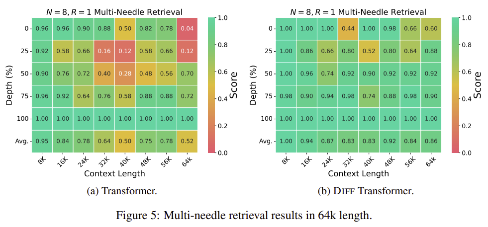
Notably, it excels in retrieving information from both short and long contexts, particularly when the data is deeply buried, and outperforms traditional Transformers in many-shot classification tasks. The model also demonstrates resilience against varying input orders during in-context learning, ensuring consistent accuracy. Plus, it boasts lower hallucination rates in summarization and question-answering tasks, indicating a sharper focus on relevant information. Finally, the Diff Transformer effectively reduces outliers in model activations, paving the way for more efficient training and inference, even at lower precision.

Another interesting consequence of Diff Transformer is that the activations and logits have outliers of smaller magnitude. This means the training would be inherently smoother leading to better convergence as observed above. One advantage of less outliers is that quantisation becomes easier and less prone to errors. You might be wondering what about compute? Well this is on average 10% slower than normal transformer owing to more computations per layer but that is fine if it leads to better qualitative performance.

Aria : An Open Multimodal Native Mixture-of-Experts Model

TLDR: 
    ARIA is an open multimodal native AI model designed to integrate diverse information modalities, offering comprehensive understanding and addressing the limitations of proprietary models.
     With 3.9B and 3.5B activated parameters for visual and text tokens, respectively, ARIA achieves best-in-class performance, surpassing models like Pixtral-12B and Llama3.2-11B, and competes with leading proprietary models on various multimodal tasks.
     The model is pre-trained from scratch using a 4-stage pipeline that enhances its capabilities in language understanding, multimodal processing, long context windows, and instruction following.

Meet Aria, a new open-source player in the AI scene, designed as a "multimodal native" mixture-of-experts (MoE) model. In simple terms, Aria can handle different types of inputs: text, images, code, and videos using a single, unified model, with no need to switch between specialized versions. Think of it like the open-source answer to proprietary giants like GPT-4o or Gemini-1.5, but with a fully transparent training recipe. While proprietary models might dominate in versatility, they keep their training methods under wraps. That’s where many open-source projects stumble, either zeroing in on just one type of input or struggling to juggle multiple types effectively. Aria bridges this gap, showing a clear path to training a multimodal native model.

ARIA is powered by a Mixture of Experts architecture which we’ve extensively covered in our blogs for DBRX, Jamba and OLMoE. Basically in the FFNN module, there are moe_num_experts (=64 here) experts out of which only a fraction num_experts_per_tok (=6) are activated aka the token is passed through only those weights. This model is narrower than MiniCPM.

Aria also has a custom-built visual encoder, which transforms visual inputs into something the model can understand, visual tokens that resemble text tokens in structure. The visual encoder, built on a Vision Transformer (ViT), divides images into patches while preserving their structure, making it flexible for different resolutions. It builds on a pre-trained SigLIP-SO400M model (same as MiniCPM-V) and fine-tunes it with Aria's unique blend of multimodal data. A projection module then converts these image embeddings into visual tokens using a cross-attention layer and an FFN, ready for further processing.

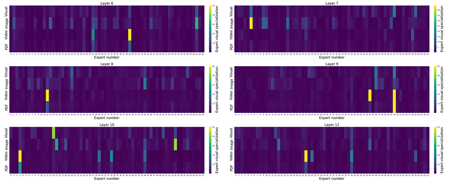
Though the model is trained in a modality independent way, few experts tend to attend to one modality more than the other. This phenomenon, commonly called as Expert Specialisation can be visualised above. Wherever you see yellow, that expert prefers that modality over text heavily aka higher proportion of image/video/visual tokens go to that expert than the text tokens.

To keep the expert workload balanced, Aria uses load balancing loss. This prevents a few experts from doing all the heavy lifting, which would cap their learning capacity. Aria also uses a z-loss to keep training stable and avoid uncertainty in predictions. You can learn more about these losses here. When it comes to text processing, it activates 3.5 billion parameters at a time out of a total of 25.3 billion. For visual inputs, a 438 million-parameter encoder takes care of turning images into tokens, handling various input sizes with ease. And for those longer tasks, it supports up to a 64,000-token context window.

Aria's training process rolls out in four stages, each one adding a new set of skills without forgetting the old. If you remember, MiniCPM also has similar stages of (pre) training.

Stage one is all about language pre-training, 6.4 trillion tokens' worth, using next-token prediction over an 8K token context window. In-context learning helps models understand tasks by using examples or instructions within the same context, improved through data clustering. By grouping similar text and packing them into sequences during training, the model learns patterns more efficiently. Inspired by Shi et al. (2023), this boosts in context learning but struggles with scalability on large datasets, leading to inefficient long-tail structures. To tackle this, a Minimum Spanning Tree (MST) algorithm clusters data more efficiently, linking similar sequences while reducing long-tail issues, making the process scalable for large data volumes.

Stage Two is where it starts to think in pictures, adding 400 billion tokens of mixed language and visual data, including image-text pairs and video descriptions. Stage three stretches its memory, extending the context window to 64K tokens through multimodal long-context pre-training, great for tasks like video analysis.

The final stage, multimodal post-training, fine-tunes its question-answering and instruction-following skills with 20 billion high-quality tokens, giving it a well-rounded boost across code, reasoning, and multimodal challenges.

Aria’s performance speaks for itself. It’s a top contender among open-source models, surpassing names like Pixtral-12B and Llama3.2-11B in tasks involving language, images, and code—all while keeping inference costs down. It even matches up to some of the proprietary heavyweights, proving its worth in complex multimodal scenarios. Aria outshines models like Qwen2-VL-7B and even proprietary options like GPT-4o mini and Gemini-1.5-Flash, especially when it comes to understanding lengthy videos and documents.

When it comes to its MoE setup, Aria knows how to make the most of its experts. The analysis shows how effectively it uses different experts for varying data types, with visual and text tokens activating specialized experts across layers. The visual specialization ratio highlights that a good chunk of the experts specializes in visual data, especially in certain layers (4, 5, 14, and 20), which are consistently active during visual tasks. This adaptability suggests that Aria’s architecture has tuned itself well during pre-training, making it ready for all sorts of visual challenges.

Le Ministraux: Ministral 3B and 8B

MistralAI released a new set of models called Minstral. ( For those interested, Ministra-ux the suffix in french is used for plural nouns in place of al suffix) This comes in two size variants 3B and 8B. Both models are said to support for 128K context length with a sliding window size of 32K. The 8B model apparently has interleaved sliding window attention. This is something we also saw for Gemma-2 family of models that we covered a few editions ago. That means, maybe more unreleased models would be trying out such techniques now.

The larger model Ministral-8B Instruct is on HuggingFace but isn’t really compatible with transformers library yet (there are converted variants to help out meanwhile). The models outperform other popular models of their own size class. But unfortunately there’s no mention of Qwen-2.5-7B. Qwen 2.5 family of models are well appreciated for their coding capabilities.

Performance of base models

Performance of Instruct models

There aren’t many first hand reviews of the model yet as it is only one day old. But this should gain adoption in the coming few days and weeks. But from the initial impressions, people claim to prefer Qwen (which btw is Apache 2.0) over Ministral. But hey it at least answered the Pound of bricks vs Kilo of feathers question properly

Q: What is heavier, a pound of bricks or a kilo of feathers?


Model: You cannot compare a pound and a kilo directly because they are different units of measurement. A pound is a unit used in the imperial system (1 pound = approximately 453.592 grams), while a kilo is a metric unit (1 kilo = 1000 grams).

To compare the two, you need to convert them to the same unit. If we compare a pound of bricks to a kilo of feathers:

- A pound of bricks is approximately 453.592 grams.
- A kilo of feathers is 1000 grams.

Given that feathers are lighter than bricks, a kilo of feathers is heavier than a pound of bricks.

These models are also available to be consumed via mistral’s platform APIs. Unfortunately the license seems to be Mistral Research License. So probably a no to enterprise use? One has to reach out to the mistral team for self deployed use. This is very different from what Mistral started out with 1y ago with mistral-7b-v0.1 promising to be open research lab :). You either die an open research lab or live long enough to see yourself become the closed lab.