
AI Unplugged 19: KTO for model alignment, OLMoE, Mamba in the LlaMa, Plan Search
Insights over Information


Table of Contents:
KTO: Model Alignment as Prospect Theoretic Optimization
OLMoE: Open Mixture of Expert Models
The Mamba in the Llama
PlanSearch: Planning In Natural Language Improves LLM Search
KTO: Model Alignment as Prospect Theoretic Optimization
TLDR:
    KTO is an alignment objective, an alternative to DPO and PPO. It builds on Human Aware Loss (HALO) of being more risk averse than gain oriented.
    KTO outperforms DPO even in low data settings. KTO doesn't really need SFT but benefits from having it. Higher the model's initial capacity, better it performs on KTO. The best part is, it doesn't require preference (pairs) data hence more robust to unbalanced data :)
Aligning generative models with human feedback has revolutionized the way we make AI outputs more helpful, factual, and ethical. Traditional alignment methods like Reinforcement Learning from Human Feedback (RLHF) and Direct Preference Optimization (DPO) have proven to be more effective than supervised finetuning (SFT) alone. However, these methods typically rely on human preferences, which are scarce and costly to collect.
KTO, a new technique inspired by the work of Nobel Prize-winning economists Daniel Kahneman and Amos Tversky, offers a promising alternative. Unlike RLHF and DPO, KTO only requires a binary signal indicating whether an output is desirable or undesirable, making it easier and cheaper to gather the necessary data for alignment. This approach leverages the principles of Kahneman and Tversky's Prospect Theory, which explains human decision-making under uncertainty.

Prospect Theory suggests that humans are loss-averse and perceive gains and losses relative to a reference point in a biased but predictable manner. This insight is crucial for understanding why alignment methods work so well. For example, given a gamble that offers an 80% chance of winning $100 and a 20% chance of winning nothing, a person might prefer a sure gain of $60 over the gamble, even though the expected value of the gamble is $80.
KTO uses this concept to inform their Human-aware loss, enabling a more nuanced comparison of data points with a reference point.

Based on this definition the paper proves how DPO and PPO-Clip are instances of HALOs (Human Aware Losses).
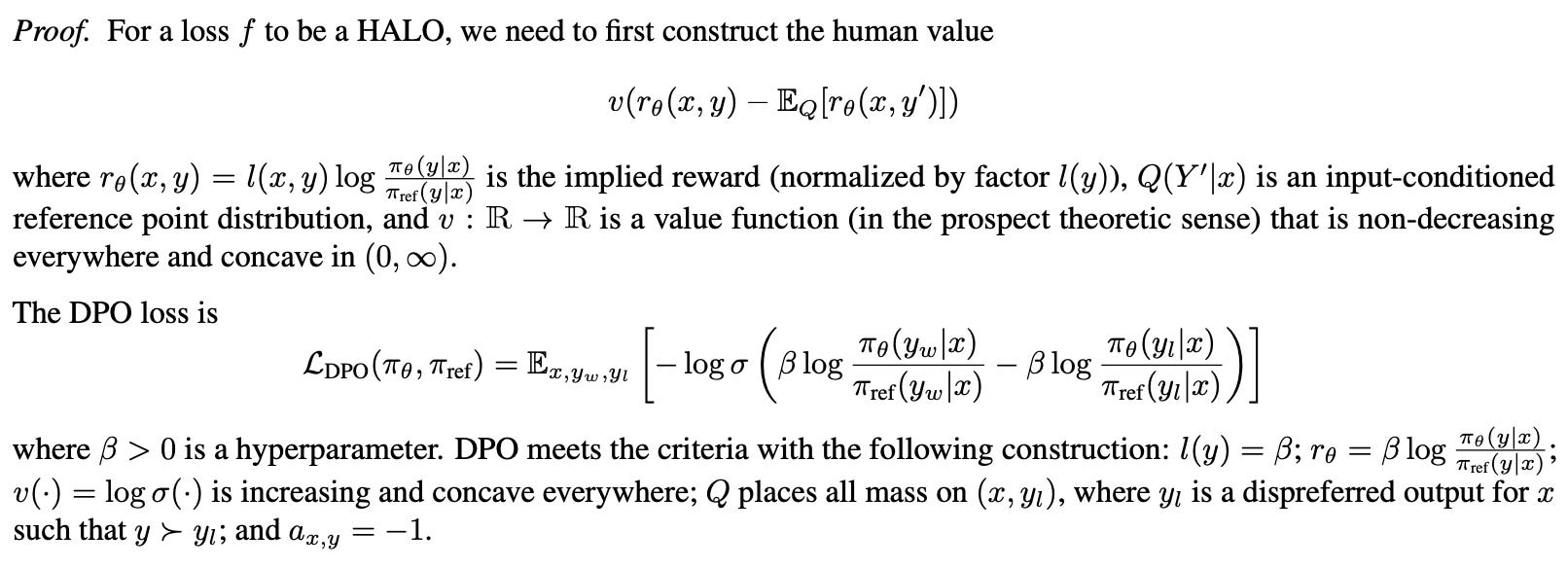
As mentioned in the proof above, just rewriting the loss function of DPO in the language of HALO proves that DPO is a HALO function.
Now, before delving into KTO, whose loss function is derived from HALOs, it's important to validate the importance of HALO over non-HALO methods. So, in the paper they performed a comparative study between some non-HALO methods (CSFT, SLiC) with HALO methods (DPO, PPO (offline)) on two model families, Pythia- {1.4B, 2.8B, 6.9B, 12B} and Llama- {7B, 13B, 30B}.
Calling PPO (offline) method PPO is somewhat imprecise, because it is offline and takes only one step, but to avoid introducing too many new terms, the paper describes it as PPO (offline). Instead of using learned rewards, we simplify even further and use dummy +1/-1 rewards for yw and yl instead.

Based on this experiment here are the conclusions:
HALOs either match or outperform non-HALOs at every scale and outperform significantly at 13B+ model sizes.
Alignment provides minimal gains for smaller models. Gains increase with more performant base models and less similar SFT data.
Our offline PPO variant, despite using simple +1/-1 rewards, performs as well as DPO for all models except Llama-30B. This challenges the focus on reward learning and shows that even basic rewards can be effective with the right loss function.
KTO derivation:
The surprising success of offline PPO with dummy +1/-1 rewards suggests that—with the right inductive biases—a binary signal of good/bad generations may be sufficient to reach DPO-level performance, even if the offline PPO approach itself was unable to do so past a certain scale. Taking a more principled approach, we now derive a HALO using the Kahneman-Tversky model of human utility, which allows us to directly optimize for utility instead of maximizing the log-likelihood of preferences.
Assumptions:
The canonical Kahneman-Tversky value function (as shown above) suffers from numerical instability during optimization due to the exponent α, so we replace it with the logistic function σ, which is also concave in gains and convex in losses.
To control the degree of risk aversion, we introduce a hyperparameter β ∈ R+ as part of the value function. (Analogous to β in DPO loss)
Rather than having just one dispreferred generation serve as the reference point z₀, as in DPO, we assume that humans judge the quality of y|x in relation to all possible outputs. This implies that Q (Y′|x) is the policy and that the reference point is the KL divergence.
Feeding all these components into the HALO definition, we arrive at the KTO loss shown below. This formulation results in a very simple expression that does not require preference data.
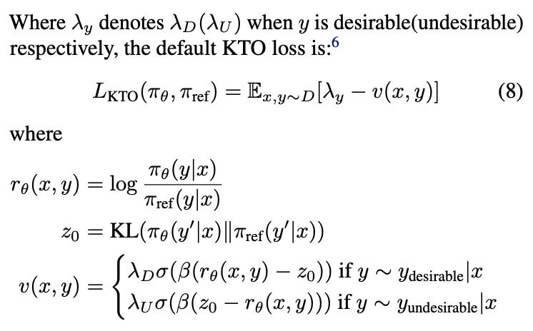
Intuitively, KTO works by penalizing blunt reward increases for desirable outputs through a rising KL penalty, forcing the model to learn what specifically makes an output desirable. This allows reward increases without raising the KL term. The non-negativity of the KL term also leads to faster loss saturation.Important points to consider before training:
The KL estimate is challenging to calculate directly due to the slow sampling process and human perception biases. To approximate the human reference point, we create pairs of similar examples and estimate a shared reference point. This biased estimate is beneficial for simulating human decision-making.

The default weighting function controls the degree of loss aversion with two hyperparameters λD, λU that are both set to 1. In a class-imbalanced setting, where nD and nU refer to the number of desirable and undesirable examples respectively, we find that it is generally best to set λD, λU such that

where one of the two should be set to 1 and the ratio is controlled by changing the other. For example, if there were a 1:10 ratio of desirable:undesirable examples, we would set λU = 1, λD ∈ [10, 10.33].
Models were evaluated against GPT-4-0613 to determine alignment quality.Apart from that, MMLU, GSM8K, HumanEval, and BigBench-Hard were used to assess model performance.

SFT+KTO and SFT+DPO were competitive at various scales. KTO alone outperformed DPO for Llama models. KTO consistently outperformed DPO and other baselines, especially on tasks like GSM8K.
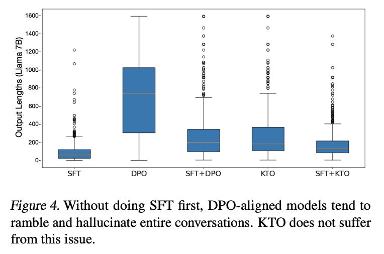
KTO-aligned Llama models without SFT were competitive with SFT+KTO counterparts. KTO alone maintained response length, while DPO without SFT led to significant increases.
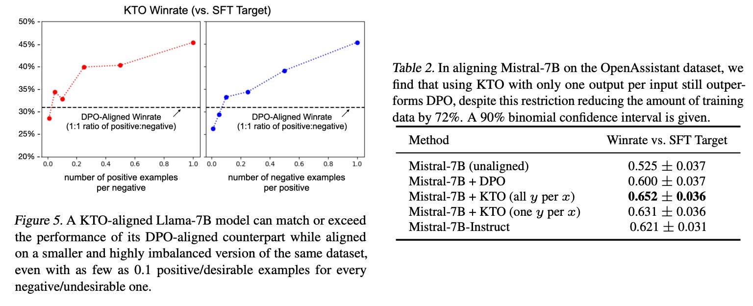
Even on discarding “desirable data” increasingly, KTO outperformed DPO on llama-7b. To validate the same, Mistral 7B was aligned using OpenAssistant data by (1) using all 2n pairs (2) using one output per input (reducing data by 72%) and the KTO variant outperforms DPO.
Modifying KTO's design can significantly impact its performance. Removing the reference point z₀, a crucial component for KTO to qualify as a HALO, led to a notable decline in performance on BBH and GSM8K. Even changes that maintain KTO's HALO status, such as removing the symmetry of the value function, resulted in significant performance drops on these benchmarks.
KTO can function without a reference model or SFT, but its performance is generally inferior to standard KTO. A memory-efficient variant of KTO can be implemented by assuming a uniform distribution for πref, simplifying the calculation of rθ − z0. While this variant performs competitively on some tasks, it is more sensitive to hyper-parameter tuning and may not always outperform standard KTO. Despite its limitations, it offers a memory-efficient alternative compared to existing approaches, as it avoids storing the reference model and requires smaller batches of data.
Why does KTO perform so well?
KTO was designed with the motivation that even if binary feedback were weaker, one could compensate with sheer volume, as such data is much more abundant, cheaper, and faster to collect than preferences. So why does KTO perform as well or better than DPO on the same preference data (that has been broken up)? Greater data efficiency helps, but it is not the only answer, given that even after adjusting for this factor in the one-y-per-x setup (By breaking up n preferences meant for DPO into 2n examples for KTO), KTO still outperforms.
The answer lies in the following prepositions and theorems:

Rather than going too much into detail of these theorems and proposition I'll summarize what are the findings from each of these:
Implicit Data Filtering: KTO tends to ignore difficult or easy examples. This can be beneficial for avoiding noisy data. However, it may lead to under-fitting complex distributions. Such under-fitting may be mitigated by aligning the model with lower β and for more epochs.
Preference Likelihood vs. Human Utility: Maximizing preference likelihood does not always maximize human utility. Reward functions in the same equivalence class can induce the same optimal policy but different value distributions.
Data Contradictions and Policy Optimization:KTO and DPO may prioritize different outputs in the presence of contradictory preferences. KTO's policy is more likely to align with the majority-preferred output.
These theoretical explanations help elucidate why KTO outperforms DPO in certain scenarios, despite the challenges associated with weaker binary feedback and noisy data.
Despite its success, KTO suggests that there is no universally superior Human-aware Loss (HALO); the best HALO depends on the specific inductive biases of a given setting. Therefore, the choice of HALO should be made deliberately rather than defaulting to any one loss function. This flexibility and efficiency make KTO a highly scalable option for aligning large language models in real-world applications.
DPO or KTO ?
With all these experiments and theoretical analysis here's a final usage guidance:
Binary Feedback: KTO is the preferred choice for binary feedback, especially with imbalanced data.
Preference Data: DPO may be better suited for noise-free and intransitive preference data, but KTO's worst-case guarantees can be advantageous in noisy environments.
Real-world Data: Most publicly available preference datasets contain noise and intransitivity, making KTO a suitable choice.
Synthetic Feedback: Even synthetic feedback can be noisy, favoring KTO over DPO in certain scenarios.
The existence of HALOs raises questions about the suitability of the Kahneman-Tversky value function for language-based tasks and the need for more tailored approaches. Future research should focus on developing HALOs that are individualized, incorporate granular feedback, adapt to various modalities and model classes, resolve contradictions fairly, work with online data, and be evaluated in real-world settings.
In conclusion, the success of model alignment heavily relies on the inductive biases of alignment objectives, which align with human biases in decision-making as explained by prospect theory. We consolidate these insights into a family of alignment objectives called human-aware losses (HALOs). Among these, the paper proposed Kahneman-Tversky Optimization (KTO), a HALO that directly maximizes the utility of generations rather than the likelihood of preferences. Despite using only, a binary signal of whether an output is desirable or undesirable, KTO performed as well as or better than preference-based methods in our experiments. Additionally, this work suggests that there is no universally superior reward model or loss function; the best HALO depends on the specific inductive biases suitable for each setting, indicating the need for continued research to identify the optimal HALO for different contexts.
OLMoE: Open Mixture of Expert Models
TLDR: OLMoE is a mixture of experts model from allenai with open weights, training code, checkpoints and logs. A few notable observations from the paper:
  0. OLMoE-1B-7B has 1.3B active params and 6.9B total params.
  1. Many small experts (64,8 active) better than few larger expert
  2. Load balancing loss and router-z loss to squish activations
  3. Truncate initialisation weights to ±3*σ=0.06 for more stability.
  4. Weight decay is applied for Embedding and RMSNorm parameters.
The original OLMo paper titled OLMo: Accelerating science of language models was a pretty significant paper at it. They went as far as releasing the training code on github. OLMoE is a natural extension to that but for Mixture of Experts. Along with that, there are also logs and whopping 244 checkpoints.
The current model, OLMoE-1B-7B as the name suggests, has 1.3B active parameters while having a total of 6.9B parameters. It is trained on a total of 5.1T tokens. The training took 10 days on 256 H100 GPUs aka 61440 H100 GPU hours. This is much more than 1.5-Pints but 1/3rd of llama-2-7B (though it was on A100). Each layer has 64 experts out of which 8 are activated. You might already be familiar with MoE architecture. But for those who are new, instead of the FFNN in a transformer block, there are Ne individual feed forward layers out of which k experts are activated. The router decides which experts to choose and the output of those experts is added in the end. We talked at length about how to understand the parameter count and active parameters in our Jamba blog.

This is how the output of the MoE mathematically looks like.

Now to make sure that all the tokens are not passing through the same experts, we have a two auxiliary losses called load balancing loss and Router-Z loss.

Why load balancing loss you ask? Because without that, there’s very high chance that all tokens end up going through same experts defeating the purpose of MoE. Introducing such a load balancing loss, almost ensures that each expert receives equal-ish amount of tokens.

As to why Router-Z loss you ask? The output of the router might cause the final logits to be very high which might cause numerical overflows. Hence to make sure that the said logits are not too high, we add a loss. This looks very much like the L2 regularisation we generally use but with a little different accumulation.

If you see, MoE reach same downstream accuracy as that of similarly sized dense model but in much much lesser training flops aka 3X lesser tokens or flops. But because of higher memory requirements, it reaches that said convergence 2x faster.

So you may ask, why 64 experts and 8 chosen instead of 8:1 or 32:4 like other models? Well they do experiment with such configuration keeping the total parameters and compute cost constant. The result is, more smaller experts are better than few larger experts. In the case of 8 experts and 2 chosen, there are 8C1 = 8 choices and that increases with increasing number of experts. From 1 out of 8 experts to 4 out of 32 experts (same ratio), there’s 10% improvement on hellaswag. But the returns diminish after 64 experts. Maybe after that point, we’re shrinking the hidden dimension way too much. Given that the hidden size is 2048, maybe going lower than 1024 is not ideal? They also observe that having a shared expert (which is active for all the tokens) is detrimental to the down stream performance.
There are generally two ways to train MoEs. One is to initialise an MoE randomly and train it from scratch. The other is to take an already trained dense model, modify the MLP to include experts and fine tune or continue training. The second one is what Mixtral uses. Hence the Mixtral-8x7B. But OLMoE goes the later route of initialising from scratch.
Now that we know things are initialised from scratch, what initialisation is it? Generally, Normal initialisation is used. Off late, Kaiming Uniform has arisen the choice of initialisation. OLMoE observes that normal initialisation with a standard deviation of 0.02 performs better if one truncates the init weights to ± 3x0.02. For the astute among you, in statistics, there’s something called Three Sigma Rule which states that 99.73% of the data points fall within 3σ or 3 standard deviations from the mean on the either side. So essentially, what you’re doing by truncating is, removing so called outlier weights.
Given all that, weight decay is a common regularisation applied for training. Embedding parameters and normalisation layers are generally omitted from this. But OLMoE chose to decay even those parameters. Apart from this, there’s another normalisation after computing Q and K. This helps stabilise the training at 10% throughput reduction. OLMoE introduces a few more metrics to understand the whole pipeline and model better.
Router Saturation: Measures how similar a router is at time step t compared to its final form at time step T. Ideally, it should keep increasing over time. This is what is observed as well. Eit is set of experts active for i-th token at t-checkpoint
\(\begin{equation} \text{Router Saturation}(t) = \frac{1}{N} \sum_{i=1}^{N} \frac{|\mathcal{E}_i(t) \cap \mathcal{E}_i(T)|}{\kappa} \end{equation}\)Expert Co-activation: How frequently pairs of experts are used together. This is per layer per router-pair metric. If multiple pairs of experts have high co-activation (close to 1.0), that means they are frequently activated together and hence can be merged into one.
\(\begin{equation} \text{Expert Co-Activation}(E_i, E_j) = \frac{N_{{E_i},{E_j}}}{N_{E_i}} \end{equation}\)Domain Specialization: Measures proportion of tokens from domain (code, conversation, summarisation etc) routing to said expert. It is observed that this is close to random (12.5%). This validates the functioning of load balancing losses.
\(\begin{equation} \text{Domain Specialisation}(E_i, D) = \frac{N^{(k)}_{{E_i},{D}}}{N_{D}} \end{equation}\)Vocabulary Specialization: Measures how often a token (from vocab) routes to a said expert. It is observed to increase as we go deeper into the network. Some tokens exclusively end up going to some said/fixed experts.
\(\begin{equation} \text{Vocabulary specialization}(E_i, x) = \frac{N^{(k)}_{{x},{E_i}}}{N_{E_i}} \space\space\space\space \text{x is from vocab} \end{equation}\)
OLMoE is a wonderful work which explores around why some decisions are taken when training MoEs and what performance gains one can expect from the same. It sort of is a good starting guide on settings for training MoEs. Really appreciate the work done by the team and then open sourcing everything is a cherry on top.
Spectrum: Targeted Training on Signal to Noise Ratio
TLDR:
    Spectrum is a way of finding which layers/modules/weights are more   important and fine tune only those. Any singular value greater than a said limit is considered signal and anything less is considered noise. The Signal to Noise Ratio (SNR) is used as a metric to determine importance.
     The method outperforms QLoRA while training on only 25% layers. In fact, one can also combine the two methods. Unfortunately there aren't comparisons to LoRA or DoRA.
It is a well known fact that not all layers in a network or LLM are equally important. Some layers change the input very little while some alter the input significantly. We’ve already talked about the same in one of our previous works on Mixture Of Depth Experts. So it might be natural to think, should I really update all the layers and weights when I fine tune something? The intuitive answer would be no given the context.
Now the question boils down to how does one figure out the layers to fine tune? You ideally need a metric which says how much information a layer or weight adds to the input. There are tonnes of ways to interpret matrices. The most natural way to analyse a matrix is by looking at its eigen values. Eigen values explain how much a matrix (eigen vector) modifies the said input. So eigen values are a proxy to how information rich a matrix is.
Each matrix can be represented as a product of orthogonal and a diagonal matrix called as Singular Value Decomposition. The diagonal matrix S’s elements are called singular values. Mathematically they are the square roots of eigen values. U and V are orthogonal aka UV=I (Identity matrix).
For large random rectangular matrices, singular values are said to obey the Marchenko–Pastur distribution. Given sufficiently large random rectangular matrix of shape (m,n), and the standard deviation σ the singular values of W are bound by
So anything which is less than these said limits can be assumed to be from noise and anything that is greater than the bound can be understood as significant enough singular values that arise from the matrix and its information itself. The code can be found here.
This gives a PSNR metric on matrices. PSNR is quite often used in Computer Vision and Image Tasks. The higher the PSNR, the higher signal is (compared to noise) indicating information denseness. So weights or modules or layers with high PSNR are “important” and contain vital information.
Given all these, you try to identify a set of layers from a network which stand higher in terms of PSNR and consider only them for fine tuning. This helps us train only those specific layers. This helps us save a lot of memory as we’d freeze the rest. Always remember, any parameter you freeze, you’d save 3x that in terms of memory if you’re using AdamW or any momentum based optimisers.

Now what does this compete against? Basically any other parameter efficient fine tuning techniques like LoRA, QLoRA and their derivatives. That is essentially what this is compared against as well. Spectrum-25% is fine tuning only 25% of the weights (the ones with highest PSNR) and Spectrum-50% is fine tuning 50% of weights.
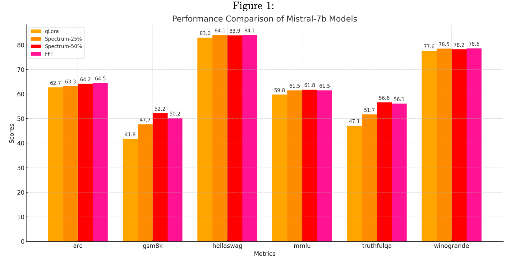
As expected, this performs better than QLoRA while being a little worse than FFT (full fine tune). But getting to those levels of accuracy with much lesser memory requirements is a good start.
This work is very similar to the works of Charles Martin at calculated content where they heavily explore Random Matrix Theory for analysing why some models are better trained than others. Do check out their wonderful content.
The Mamba in the Llama: Distilling and Accelerating Hybrid Models
TLDR: The paper discusses distilling a large pre-trained Transformer model into a linear RNN. Few notes from the paper:
  1. Aims to map Transformer weights to linear RNN weights.
  2. Relationship between softmax attention and linear RNN.
  2. Adapt Transformer decoding techniques.
  4. Authors distill LLMs Zephyr 7B, Llama3 Instruct 8B into hybrid models.
  5. These hybrids, especially the 50% attention variant, outperform or match the original models.
Guess, after all our previous editions, we need not mention the success of transformer models, especially in language modeling. But we have also the rise of Mamba models, and its upgraded version, Mamba2. We have also seen hybrids like Jamba1.5 in our last edition. Not to mention again; the main difference between these two is that the computation grows quadratically with sequence length in transformers, whereas Mamba models scale linearly. This makes them a go-to choice for handling longer sequences efficiently, often generating sequences up to five times faster, especially when transformers hit a wall with the KV cache. This is handy, especially in tasks such as reasoning over long documents.
This paper takes a different route: distilling a large pre-trained Transformer model into a linear RNN. It tries to tackle two challenges:
How do you map those hefty pre-trained Transformer weights onto linear RNN weights for distillation?
How do you adapt transformer inference techniques, such as speculative decoding, to this new architecture?
First up, the mapping challenge. In Transformers, attention is computed in parallel across multiple heads to capture relationships between different parts of the input.
where Q, K, V are query, key and value matrices, m is the mask (1 if s <= t else 0). The linear RNN, on the other hand, takes the following form, where h is the hidden state and A, B, C are the parameters.
Despite the visual difference, there is a natural relationship between these formulations. If we ignore the softmax attention, i.e linearizing it, we can convert it into linear RNN form.
In analogy to linear RNN,
So, if we the input is i , the parameters A, B, C would then be
Note that the hidden state above has a dimension of Nx1 and hence naively applying this transformation leads to poor results. It produces a degraded representation of the original model, as the softmax nonlinearity is critical to attention. However, there are other works that have utilized kernel methods to improve this approximation. The general idea is to replace the softmax kernel by another kernel.
where φ that needs to satisfy certain properties. There is an interesting approach called Hedgehog Attention, which simply uses a MLP as the φ. Back to the paper, it does this using the Mamba framework. The new model doesn’t capture the exact original attention function, but instead uses the linearized form as a starting point for distillation. Mamba leverages a continuous-time state-space model (SSM) to parameterize a linear RNN during runtime, described by a differential equation:
Failed to render LaTeX expression — no expression found

To make this work for discrete-time problems like language modeling, they use a neural network (MLP) to generate a sequence of sampling intervals ∆t and samples of the signals at these time steps. Given T samples of B, C, Mamba approximates the continuous-time equation using a linear RNN. The only extra parameters to be learned are the sampling rate ∆ and the dynamic A. These new parameters guide the linear RNN via a discretization function, which gives you the new matrix-valued linear RNN. This algorithm feeds the standard Q, K, V heads from attention directly into the Mamba discretization, and then applies the resulting linear RNN.
Now, onto the second challenge: Transformer models generate sequences one token at a time, which creates a bottleneck because the model has to wait for each previous token to be fully generated before moving on to the next one. Speculative decoding tries to speed things up by predicting multiple future tokens in advance and then verifying these predictions. This process relies on two models:
Draft Model: Quickly generates potential future sequences.
Verification Model: Checks if these generated sequences are valid.

The idea here is to let the draft model generate several possible sequences ahead of time, and then the verification model confirms which of those sequences are correct. If a sequence passes verification, it speeds up the overall process. If not, the system goes back to the last verified state and tries a different sequence. You can take a look at one such, S3D, here. This is pretty straightforward in transformers because the KV cache, which is basically K[1:t] and V[1:t] for t tokens, allows you to rewind to any point in the sequence (for t’ ≤ t, this would be K[1:t’] and V[1:t’]). But with linear RNNs, there’s just a single hidden state (h[t]) at any given moment, so we need to be smart about caching to avoid excessive memory usage (we don't wanna store h[1:t] as that would essentially make it the same as transformers). This is also simple though. We store the hidden state of the last verified token, generate new sequences (they use a multi-step generation kernel for this), verify them, and then update the hidden state corresponding to the last accepted token. So at any point in time, we only cache the hidden state of the last verified token.

Two LLMs - Zephyr 7B and Llama3 Instruct 8B - were distilled into hybrid models using a mix of linear RNN (Mamba and Mamba2) and attention layers. These hybrids came in different flavors: 50%, 25%, 12.5%, and 0% attention. The distillation process itself was done in three stages: seed prompts, supervised fine-tuning, and distilled alignment. When put to the test on chat benchmarks like AlpacaEval and MT-Bench, the hybrid models (especially the 50% attention variant) held their own, performing as well or better than the original teacher models. On the other hand, the pure RNN model (0% attention) fell short in accuracy, but interestingly, the hybrids outshined even large transformer models like Falcon Mamba. General benchmarks using the LM Evaluation Harness also showed the distilled hybrids doing just as well as top-tier linear RNN models on tasks like WinoGrande, ARC-Easy, and TruthfulQA. Hybrid speculative decoding led to speedups of over 1.8x using Zephyr and Llama hybrids. However, when they tried this with larger draft models for Llama, the gains were more modest. Looks like the next step will be about fine-tuning these draft models to squeeze out more efficiency.
Planning In Natural Language Improves LLM Search For Code Generation
TLDR: PlanSearch is a search-based method for improving code generation in large language models (LLMs). Unlike traditional methods like beam search or repeated sampling, which focus on output diversity, PlanSearch focuses on generating diverse natural language "plans" before converting them into code. It does this by making observations about the problem, generating multiple ideas, and translating them into code. The approach was tested on benchmarks like MBPP+, HumanEval+, and LiveCodeBench, showing strong performance for solving complex coding problems.In machine learning, scaling up learning and search are two key ways to boost performance. Large language models (LLMs) have shown that scaling up learning works wonders. But when it comes to scaling up search techniques for LLMs, the results haven’t been as promising, even though search methods have been a game-changer in other machine learning fields (remember Alpha Go?).
When we talk about "search" here, we’re talking about using extra computational power during the model's inference phase to squeeze out better performance. PlanSearch is one such approach; improving search specifically for code generation using LLMs. One of the big hurdles for using search in code generation is that LLM outputs often lack variety. So far, approaches like beam search or repeated sampling at higher temperatures have been used to churn out multiple candidate solutions, hoping that at least one is spot on. But these methods have stuck to pretty basic sampling techniques without really tapping into richer search spaces.
To step things up, certain approaches mix repeated sampling with filtering algorithms (verifiers or reward models, for example). This method, called best-of-n sampling, picks the best result from multiple outputs. Fun fact: some studies show that repeated sampling can even beat out single large-model outputs when used smartly. There are also other exciting new approaches, like "Tree of Thoughts" and "Reasoning via Planning," that have taken a search-like approach to reasoning. But they haven’t been tested on complex tasks just yet.

PlanSearch takes things a step further by searching through natural language-based plans before generating the code. This helps generate more diverse, better results since it expands the range of ideas. While repeated sampling zeroes in on output space, PlanSearch targets the idea space - resulting in higher pass rates for tough problems.
The idea is to explore multiple plans and then convert those into final code solutions. But one tricky part of any search algorithm is figuring out what exactly to search over. The magic seems to lie in creating the right "solution sketch"- a natural language description of the program. Backtranslation steps in here. It’s about taking correct code solutions and turning them back into natural language sketches using a language model. The paper’s experiment generated 1,000 code attempts, and the correct solutions were turned into sketches.
Here’s how PlanSearch works:
Prompting for Observations: The model is first asked to make observations about the problem. These act as hints that guide the idea search. Typically, 3-6 first-order observations are generated. Then, all possible combinations (of size at most 2) from these observations are created for the next step.
Deriving New Observations: The model is now prompted with the problem and each combination of observations. It’s asked to combine and refine these observations to generate second-order insights. Now, these observations might not always be spot-on, but the goal is to push the model to explore a wider range of possibilities. You could theoretically do this an unlimited number of times, but the authors stopped after this stage.
Observations to Code: Once observations have been generated, the model is prompted to turn them into natural language solutions. For each idea, the model generates an additional idea by assuming the first one is wrong. This doubles the number of ideas being considered. Then, these natural language solutions are translated into pseudocode and eventually into Python code.
The model was asked to create its own sketches for problems in the LiveCodeBench dataset. For each problem, multiple ideas were generated, and the model took a crack at solving them. The verdict? Generating a solid idea or sketch is key to solving the problem, and the quality of that sketch can make or break the solution. So, improving the sketch generation process could massively up the model’s game in solving coding problems. A key point to watch out for is ensuring that when the pseudocode is converted to Python, the model doesn’t lose track of the earlier observations - otherwise, errors can creep in.
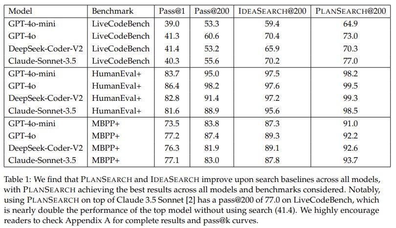
PlanSearch is evaluated for code generation across three key benchmarks: MBPP+, HumanEval+, and LiveCodeBench. Both MBPP+ and HumanEval+ are commonly used, but they've been upgraded with more test cases to better fend off reward hacking. Then there's LiveCodeBench, which is geared toward more advanced competitive programming challenges, requiring solid reasoning skills. In the experiments, the generated code had to follow strict formatting and pass every test case thrown at it. Models were cranked up with a temperature setting of 0.9 and a top-p of 0.95. The search methods tested included Repeated Sampling, IdeaSearch, and PlanSearch, with performance measured using pass@k. One cool thing to note: public test filtering (which weeds out code samples that already pass initial tests) cut down the number of submissions needed to hit high accuracy. For example, PlanSearch hit 77.1% accuracy on LiveCodeBench with only 20 submissions, compared to 77.0% with 200 submissions when filtering wasn't used.
 | A guest post by
|