

AI Unplugged 13: Qwen2, DiscoPOP, Mixture of Agents, YOLO v10, Grokked Transformers
AI Unplugged 13: Qwen2, DiscoPOP, Mixture of Agents, YOLO v10, Grokked Transformers
Insights over Information


Table of Contents:
Mixture of Agents
Grokked Transformers are Implicit Reasoners
LLMs invent better alignment algorigthms
Qwen 2
YOLO v10
Mixture of Agents
Together.ai released a new paper called Mixture-of-Agents Enhances Large Language Model Capabilities and a blog associated with it. Here they explore the case of using multiple LLMs at once.
If you have ever used ChatGPT’s custom GPTs there’s a custom GPT called Advisory board. The basic idea is, let GPT enact different characters and finally evaluate the whole response. So we’re explicitly making the model think in multiple perspectives and answer a simple or a complex question. Now that if we don’t rely on a model to produce different outputs but use different models altogether? That is almost what this paper explores.
Now say 3 models generate outputs to a given text, how do you then choose the final output? There are two immediate ways we can do this. One is to make the LLM choose which model’s output is the best and consider that as the output. Second is to as the model to look at all the previous models’ outputs and generate an output considering everything.
So once in the first layer, each model generates its own output of the initial system prompt, for the 2nd set of models, this is the prompt they use. The model is fed the outputs of models in the previous layer.

Now you must be wondering what a “layer” is. It is basically one pass through all the models. Now why is there only one model in the final layer (layer 4)? After gathering info from (say 3) models from the penultimate layer, all you need is one model to look at them to produce the final output.

Why only 4 layers? They have experimented with few different configurations. Layer 4 is where you see convergence. And this is consistent across different models like Qwen, Mixtral, LlaMA and even GPT-4o.

You might be wondering why go through all the hassle? Why invoke multiple LLMs for just a single prompt and make things super complicated and resource intensive? The answer is, as you might have guessed, improving the model’s performance. This method improves the SoTA on Alpaca eval by 8% taking it to 65.7. MoA lite is basically 2(+1 final model) layers instead of 3(+1). with GPT-4o means the final model (in layer 4) is GPT 4o, by default Qwen-1.5 110B chat is the final model.

They provide cost analysis for the same. Because they use Open Source models only, the cost is of the inference provider (together ai in this case) and GPT-4o’s pricing is from OpenAI. But what surprised me is somehow this is less tflops to compute than GPT4o? They consider rumored 8x220B for GPT4o.

It is definitely an exciting direction to research in. But the cost is way too much. Now what one can probably try is, use small open source models to reciprocate the same. And maybe in the 2nd layer and final 4th layer, use bigger models? How does quantisation effect this? Can we do speculative decoding on the concatenated output? All of this just to save on cost. Another interesting thing to study would be how much is this improvement dependent on the models having great prior capabilities? Like putting 5 mathematicians in a room and asking them to discuss and solve a problem can be helpful while having 5 math illiterates can’t give you any significant improvements.
Grokked Transformers are Implicit Reasoners
If you were ever wondering about what and how transformers learn and what would happen if you go beyond convergence, this is the paper to look at. Grokking means understand something intuitively aka “Just Get It” types like it was meant for you. So what does grokking in terms of neural networks mean? It essentially means the same thing. Instead of memorising or overfitting, the model just fully understands the “data” and patterns in it. What does that imply? A perfect model would mean perfect eval accuracy.
If you take your mind back to the days when you were learning ML, you’d remember that if you train a model too much, you tend to overfit. The model just tends to remember stuff from training data and not understand the patters at all. But recent works have explored the concept of training beyond overfitting. One such work which is (orthogonal to the one we’re talking about) Deep Double Descent. It is a phenomenon where over parametrisation, while overfitting on data, gets better if you continue training.

But in the context of the current paper, we’re not very concerned with model sizes. We’re concerned about training steps/time. How do models behave when you train them way beyond convergence (on train accuracy)? Studies have shown that models generalise amazingly well after that point. The point where train accuracy touches 100 is called the Grokking point. On small toy datasets like Modulo Arithmetic, upon grokking, you start to see patterns in embeddings/activations like shown here.

Now given the background in terms of neural networks, the question is begging to be asked. Do transformers exhibit the same property? If yes what can we infer from that? But training for 10^6 steps is a lot. And to study and understand something, its always better to start from the basic units. Hence the authors chose a small model with same architecture as GPT-2 (not the same weights ofc). Now that model is chosen, how do you choose a dataset? Ideally we’d need something small but with ample number of examples. Reasoning has been a pretty week leg for LLMs especially multi step/hop reasoning. Hence we’d tackle the same. Here’s how Mistral faired in a simple question. Look at here for more examples like Claude and Reka.

The data is of two kinds. One is for composition where given two logical statements, the model is expected to compose the two and come to a conclusion. For example, “Sachin is cricketer”, “Cricketers are athletes” are two statements called Atomic facts, the composition would be “Sachin is athlete”, called Inferred Fact. The second type of data is comparison. Given two pairs data points which have a value attached to them (or any relation), the task is to find the transitive relation. For example, assuming that we have A,B,C have values of 4,7,9 and given A<B and B<C, we can infer A<C. And taking this a step further would be not associating any values but abstract relations.
The data is then split into two groups where a few relation pairs or atomic fact pairs are withheld from the training set. The curious thing here is, out of distribution (those withheld from training set) test accuracy doesn’t increase for compistion while it does reach 100% for comparison.

Now the question arises, what is the split between Atomic Facts and Inferred Facts in the training data? They do experiment with the ratio and the whole dataset size as a whole. The conclusion is data set size has much lesser impact than the said Ratio. And as expected, having more Inferred Facts in the training data helps the model generalise better.

To understand which layers impact the output and what information is processed by which layer, the authors perturb the activations and see the causal effect on the output. This results in pretty interesting findings. Here, (h, r1, r2) is the composition relation like (Barack, wife, born in) and the expected answer is (as shown in above image) is 1964. For comparison, (a,e1,e2) is (Age, Trump, Biden) and expected output is “Younger”.

As you see, for composition case, there’s very very high causality between 5th layers r1 and r2 activations and the final output (greener in the grid). The authors observe that initial layers (layer 0-4) retrieve the first Atomic Fact and store the Bridge Entity (Michelle) in [5,r1] aka the activations corresponding to 2nd token in 5th layer. The later layers (5-8) fetch the second atomic fact and store the tail (1964) in the output state [8,r2] aka last index of 8th layer. The problem here in case of Out of distribution generalisation is, for the relations that aren’t seen as second hop in the training data, it doesn’t even know to “fetch” the second-hop relation to the 5th layer (even though it remembers it). Now if fetching the 2nd fact itself takes till later layers, when is it even gonna process that info? :)

Now in case of Comparison, the model stores the label corresponding to inequality (like <, =, >) in [7,a] aka penultimate layer’s first token activation. Similar to above, [5,e1] (5th layer activation corresponding to 2nd token) stores value corresponding to e1 aka v1 parallelly fetching v2 to [5,e2] aka 3rd token’s activation in 5th layer. Now irrespective of whether it has seen the e2 relation or the v2 value in 2nd fact, it will definitely fetch the value to [5,e2]. And hence comparison is done in later layers and the model can generalise to unseen attribute(e) values(v).

As to how this fares against big LLMs, because we can’t train them on the data, they do RAG and In Context Learning to evaluate the models. The evaluation is done on an extension of Comparison task. There are only three possible labels (aka the tokens corresponding to <,=,>). So a random guess would be 33% likely to succeed. But the so called SoTA models suck at this. It highlights two points. These SoTA models are really really bad at two(multi) hop reasoning. This table also highlights the difference between parametric memory (where things are memorised in weights) as opposed to in context memory (where things are to be memorised in context aka via activations and hidden states).

This is pretty interesting area of research. It aims to decipher LLMs, how they react to over training. Maybe we should do away with the term over training. The theory is that, at initial stages, model tends to memorise facts. But with weight decay which incentivises models to not over complicate, the models tend to Understand or Generalise more than memorise. In fact, the initial stage of memorising would need parameters equivalent to information in all the atomic and inferred facts combined. For Generalising, all you need is to memorise initial atomic facts and some relations.
LLMs invent better ways to train LLMs
LLMs have come a long way in the last few years. From being unable to write coherent sentences to being able to complement humans. Of course with more and more emerging capabilities, we start to wonder, what can or can’t LLMs do. They’re just super sophisticated parrots that just spit out the most probable word without really knowing it right? Well, on one side are people who believe this and claim that LLMs can’t discover or invent new things. While on the other side, people try to push the boundaries of what is possible with LLMs.
sakana.ai falls into the latter category given their line of work. We’ve previously featured their work on Model Merges which the academia/industry was not actively exploring yet the open source community showed it to produce good results. If you remember, they were able to beat all the math and Japanese language models on Japanese and Math tasks with evolutionary model merges. Now they’re back again exploring another side of the LLM story. To be precise, they explore if LLMs can invent/discover better ways to train LLMs (models in general). Sounds very much like the episode from Silicon Valley ig?
The problem they want to tackle is alignment. RLXF(X=Human/AI/…) has been an incredibly powerful technique to align or steer the model towards human values. PPO was/is the gold standard. But the problem is, Reinforcement Learning objectives are hard to train. DPO came along giving tough challenge to PPO. In fact, we covered a recent work comparing the two. There are other algorithms like KTO which try to tackle the alignment loss/objective. But what if we don’t want to manually go about discovering things? What if we let an LLM come up with an objective for the same?
But LLMs are notoriously resource heavy to train/fine tune. So first we need to explore the feasibility of models coming up with new loss functions. The team behind the paper used ResNet-18 training on CIFAR 10 as the case study. The results looked promising. The objectives LLMs proposed got better over generations.

So how does one go about this? They prompt the model asking it to output a loss function taking in the log probs of chosen and rejected samples wrt the current policy and the reference policy and it is expected to output the final scalar corresponding to the loss objective. Given an example of the starting where DPO’s code is provided in the context. Now once it suggests a method, they go ahead, try it out and get the metrics wrt the suggested loss. They take that whole information and try to pass it to the model’s context (they pass each of the previous generations’ codes) and ask it to generate a new function again. The thought in the output makes the LLM think before it starts to write code and hence has better chances of producing correct and coherent code. Something like Chain of Thought prompting.


They train gemma-7b model on argilla preference dataset. So across generations, the model’s suggested code gets better in terms of MT-Bench scores. They let the model suggest over 100 such objective functions and pick the best 4-5 among those and present their results. Thus suggested loss functions, comfortably outperform the best human designed ones like DPO and KTO.


After training on the said data, they also evaluate how the model on other tasks/benchmarks. The results do hold up for Alpaca Eval. Note that LC here stands for Length Corrected. Alpaca Eval asks GPT to rate the outputs of the models. So GPT is known to prefer longer outputs so Alpaca-LC compensates for that. The Log Ratio Modulated Loss LRML objective is dubbed as DiscoPOP (Discovered Preference Optimisation). And it looks something like this…
def log_ratio_modulated_loss(
   self,
   policy_chosen_logps: torch.FloatTensor,
   policy_rejected_logps: torch.FloatTensor,
   reference_chosen_logps: torch.FloatTensor,
   reference_rejected_logps: torch.FloatTensor,
  ) -> torch.FloatTensor:
        tau = 0.05
        pi_logratios = policy_chosen_logps - policy_rejected_logps
        ref_logratios = reference_chosen_logps - reference_rejected_logps
        logits = pi_logratios - ref_logratios
        logits = logits * self.beta
        # Modulate the mixing coefficient based on the log ratio magnitudes
        log_ratio_modulation = torch.sigmoid(logits / tau)
        logistic_component = -F.logsigmoid(logits)
        exp_component = torch.exp(-logits)
        # Blend between logistic and exponential component based on log ratio modulation
        losses = logistic_component * (1 - log_ratio_modulation) + exp_component * log_ratio_modulation
        return losses
The loss is basically a temperature scaled, linear combination of DPO loss and sigmoid. Pretty cool. As from what it appears like, the model mixes and matches a few techniques that are already known in the ML field and tries to come up with a new loss combining those and it works pretty pretty well. They also compare how the new loss and its gradients behaves in comparison to DPO loss.

As the beta parameter increases, the LRML loss converges towards DPO. After all, its a linear combination. And irrespective of beta, the biggest difference in the losses is observed when the logits are around zero. And the gradients around zero are significantly higher. Maybe this disincentives the logits from being around zero? But that makes little sense to me. I’ll update if I find an intuitive reason as to why this works. Also the loss is better than DPO at any given KL divergence. Note that KL divergence in RLHF is used to make sure that aligned model’s outputs don’t deviate too much from pre trained model resulting in reward exploitation and hallucinating.
But this an exciting area of research nonetheless. The models already seem to have good understanding of a lot of concepts. So its not surprising that mixing and matching few things from the first principles leads to good results. In fact, I tried mixing a couple of first principles to initialise LoRA A,B matrices differently and the results turned out to be pretty amazing. So All Hail the First Principles.
Qwen2
Qwen is a series of models from Alibaba cloud which perform exceptionally well on benchmarks and are go to for a lot of people’s fine tunes. It is so well performant that in NeurIPS LLM Efficiency challenge 2023 challenge, a lot of people’s initial model was Qwen-14B. It was so good that it outperformed LlaMA 30B on MMLU and such tasks. In fact, it was the model that even I used for my submission which ended up in top 10 :)
Qwen team also released an intermediary checkpoint called Qwen-1.5 which improved upon Qwen but now Qwen 2 is out in full we no longer have to deal with semi trained checkpoints. This generation of models come in 5 size variants. Qwen2-0.5B, Qwen2-1.5B, Qwen2-7B, Qwen2-57B-A14B, and Qwen2-72B. Unfortunately there is no 13-14B variant unlike last time. That size is perfect for LoRA fine tuning on 40GB GPU and QLoRA on 16GB GPU. Note that whenever you see a model name having “Name-XB-AYB” as in case with Qwen2-57B-A14B, it stands for a total of XB (57B) parameters while YB(14B) parameters are active for inference. That gives it away that it is a MoE model. We talked in detail about how to calculate these numbers when we uncovered Jamba, please take a look after this.

Coming to the changes, Qwen2 is trained on 29 languages incl English and Chinese. The context length is now extended from meagre 2k to 128k (32k on training but 128k by rope extension) unlike some recent models with meagre 8k. Looking at you LlaMa-3. The small models have Tied Embeddings which ties Embedding matrix and Unembedding matrix (lm_head) so that one is the inverse of the other. All the models now have Grouped Query Attention (GQA) which you can understand as num_attention_heads and num_key_value_heads are different. There also seems to be sliding window support now. Apart from that I don’t see any differences. Also I couldn’t find info about how many tokens these models are pre trained on. I asked in Qwen’s discord and they mentioned it is over 7 trillion which is half of that of LlaMA3.

Coming to the performance, Qwen2-72B comfortably outperforms LlaMA3-70B in synthetic benchmarks. But these numbers are numbers. How does this perform on our usual Pound of bricks vs Kilo of feathers question? Well it aces that question. Even on trying to put it off, it stands its own ground well.

And like every other model, it fails the Yann Le Cunn’s 7 gear problem. I tried to help it think otherwise without explicitly telling it but it didn’t help at all.

Qwen also outperforms LlaMA3 on coding fronts in almost all popular languages. The story is the same for math. Initially, I thought maybe bigger vocabulary helped Qwen, but with llama3 also having 128k vocab, that difference isn’t the reason. Maybe, multilingual data especially languages like chinese where tokens stand for some semantic meaning helps (this is just a weird hypothesis) as another such series Yi out performs LlaMA.

But LMSys chat arena ranks qwen2-72B instruct below llama3-70B. And this happens consistently across Coding, English, Long query etc. And the same is the case with OpenLLM Leaderboard. So that is one thing to make note of.
Also no more of c_attn, c_proj, w_proj like Qwen. All the layer/module names are consistent with llama like q,k,v,o_proj and up,down,gate_proj :). Also unsloth already has support for Qwen2 thanks to being similar in architecture to llamas and mistrals. No more need of llamafy-ing qwen like old to make it behave well with fine tuning frameworks. Personally qwen2 is exciting except for the missing 13-14B sized model.
YOLOv10 Real-Time End-to-End Object Detection
Imagine swiftly identifying and pinpointing objects in real-time. YOLO models have been at the forefront, mastering the balance between computational efficiency and detection prowess. YOLO stands for You Only Look Once. That is how you process frames/images, cuz you can only look at them once. In the world of computer vision, there is something called bounding boxes which are rectangles (box) around an object in the frame.
The models initially predict a set of bounding boxes, multiple around a single object often referred to as One-to-One Matching. And then, iteratively find the one with the highest confidence to consider that as possible final output. This is called Non Maximum Suppression (NMS). The problem is this is expensive. The other approach is One-to-One Matching which eliminates the problem of NMS but another issue arises where if the model is possibly thinking of multiple labels for a single object, it might not be completely sure as to what to output leading to reduced accuracy.
So why are we talking all this? What is in it for YOLO v10? Well if it wasn’t yet obvious, YOLO v10 incorporates both to reap the advantages of both while complementing for the drawbacks of each. During training, we use both to improve accuracy (as compared to One to One) and at inference, we only use One to One matching for speed. They called this as the Dual-Head model.

Take a peek at the picture up there - it lays out the whole YOLOv8 architecture. At its heart is the CSPLayer_2Conv module, aka C2. This module is crucial for building up features in the backbone and then bundling them all together in the neck. CSPNet was designed to tackle the issue of redundant gradient information in networks like ResNet and DenseNet.Basically because each block is stacked upon another, in ResNet and DenseNet, the gradients would be heavily correlated. In ResNet due to skip connections. So instead of just having skip connections, it adds another block of processing (as you see on left branch). Hence each layer’s modified-skip connection would have gradients dependent on their corresponding branch weights. Usually, its faster version, C2f, is used to enhance efficiency.

And then there’s Spatial Pyramid Pooling Fusion (SPPF). By pooling at different scales (aka diff resolutions of the same image), it helps the model recognise features at various levels of detail. This is especially useful for object detection, where detecting objects of different sizes is important. Each head in this architecture corresponds to an output in the one-to-many assignments.

YOLOv10 builds on this strong base but with some killer upgrades:
Lightweight Classification Head: The classification head (predicts the class label for given object) now features two depth-wise separable convolutions and a sleek 1x1 convolution, whilst maintaining the regression head (predicts the size and shape of the bounding boxes) complexity for peak performance.
Spatial-Channel Decoupled Downsampling: Standard 3x3 convolutions with a stride of 2 are replaced by point wise convolutions to adjust channel dimensions followed by a spatial downsampling depth wise convolution.
Large-Kernel Convolution: Large-Kernel depth wise convolutions are selectively integrated into deep stages to enhance context capture.
Partial Self-Attention (PSA): Kicks in for later stages. Basically in the final stages, they add Multi Head Self Attention to further improve the flow of information.
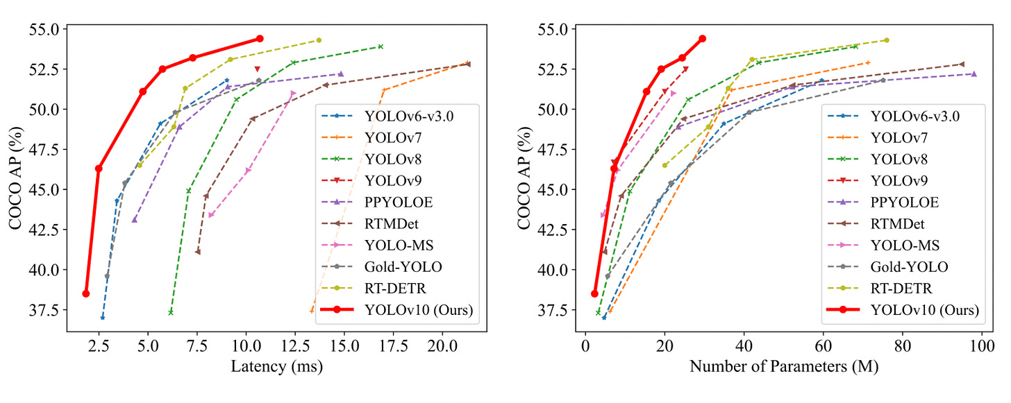
Now onto the results.

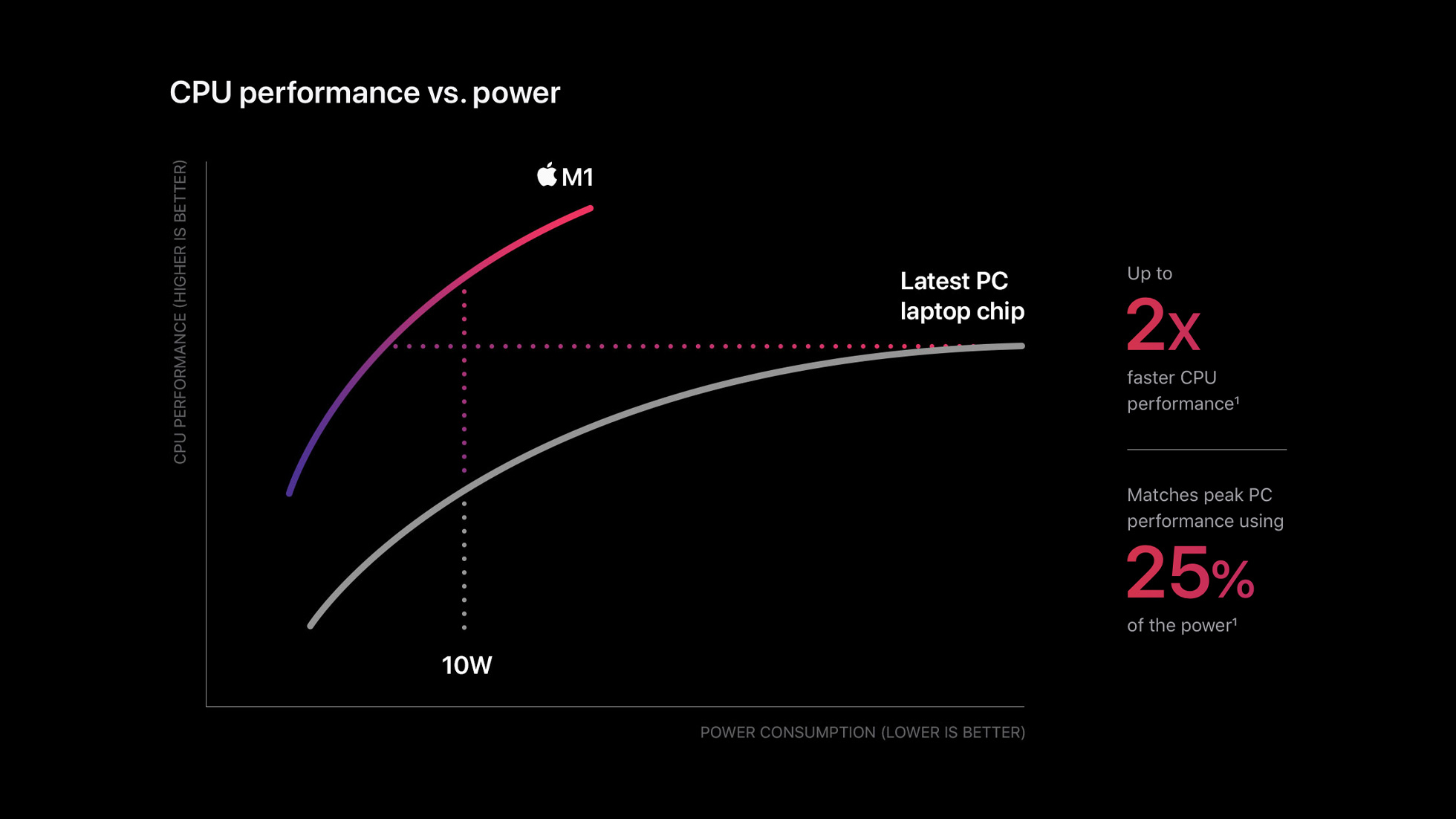
The model comes in various different sizes and ofc the bigger models have better performance at the cost of latency. As to results in terms of how it compares to other vision models, this has better latency at any given accuracy and better accuracy at a given latency. Looks very much like the graphs Apple showed when they launched M1


 | A guest post by
|
 | A guest post by
|