


AI Unplugged 12: MoRA. DPO vs PPO. CoPE Contextual Position Encoding. S3D Self Speculative Decoding.
Insights over Information


Table of Contents:
MoRA: High rank updating for PEFT
CoPE: Contextual Position Encodings
Is DPO Superior to PPO
S3D: Self Speculative Decoding
MORA: High rank updating for PEFT
Parameter Efficient Fine Tuning or PEFT is a way in which we update a model in a parameter efficient way, ie training only a few number of parameters. There are various such approaches proposing different mechanisms from Adding new layers to Inserting layers in between to training a subset of layers to LoRA. LoRA has been the most used PEFT method of all.
LoRA adds a trainable adapter where we decompose the matrix into 2 matrices of smaller rank. For a given W ∈ ℝ(m,n) , we hypothesise that the updates in fine tuning are of low rank and hence ΔW can be factored into two low rank matrices A and B of dimensions (m,r) and (r,n) where r < < m,n. So the parameters we update is very small.
There are many proposals to improve LoRA like DoRA, VeRA, LoRA+ which change one aspect or the other of LoRA. But the fundamental hypothesis is still the same that weight updates are of low rank. But what if they are not? In fact, they generally are not. We talked about a comparison between LoRA and full fine tune in an earlier blog
This is where this paper comes in. But wait, with rank, the number of parameters increase. So how can something be low parameter yet high rank? In this context, high is a relative term. Generally, when training LoRA, the number of parameters is r(m+n) and if the update parameters are fixed, the maximum rank is when we have a square matrix of updates [ a+b >= 2√(ab) ] which turns out to be . So if we somehow make the updatable parameters a square matrix, we’re good to go.

But for that to happen, we need to get the input from size m down to r somehow. aka compress the input. There are a few ways to do this. One is to just trim the vector and ignore some features. But we’d then lose information. So the other way is to say average every m/r values into one so the resulting is of size r. Or you can also define a set of indices per output dimension which you want to average over. Now the task is to decompress the r sized vector into an n sized input. This is basically done by inverting the previous step and define set of inverse indices.
One thing you should note here is that, the transformations, whatever we apply to shape and reshape the input has to be input independent. Thats the only way which would allow us to merge the new adapter weights back into the original after training finishes. Merging is essential is keeping the latency down when deployed for inference
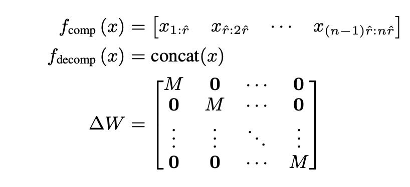
Now given all this, one additional thing they do is take a leaf off RoPE and add rotation for the groups to incorporate a little more information. So basically you rotate each of those Ms by diff angle.
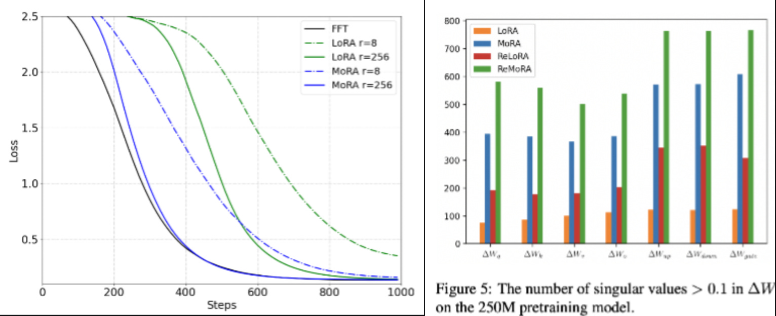
Coming to the results, they test on dataset with UUID pairs. So at test time, they’re basically evaluating the model’s ability to memorise things. As you see in the losses, MoRA converges faster than traditional LoRA. It looks very very close to full fine tuning. And if you see the number of eigen values greater than a threshold (0.1), you see that MoRA is indeed higher rank than LoRA in general.
ReLoRA is a technique where you do LoRA and merge the weights into the model, then re initialise the LoRA weights and re-train them. This MoRA can be stacked on top of ReLoRA to create ReMoRA and they do compare these two as well with same findings. They also compare their results to other techniques like LoRA+ and DoRA where this technique outperforms them.

Though these LoRA alternatives are coming out every now and then, the adoption hasn’t been as rapid and widespread as LoRA. Maybe people are really happy with what LoRA gives them. One thing is, the choice of compression and decompression functions are still not thoroughly explored. They do compare their methods against truncation and averaging but one can possibly create better pair of functions.
CoPE: Contextual Position Encoding
Position encoding is one of the most weirdest thing in Transformers. There’s a very very good reason to have position encodings. If you think about it, Attention mechanism is position equi-variant. For eg, for the sentence India defeated Australia and for the sentence Australia defeated India, the queries, keys, values would be exactly the same (but in different permutation). So to give models an understanding of what preceds what, we Add something called Position Encoding to the vectors (queries generally).
There are many types of position encodings. The OG from Attention is all you need was add Sinusoidals of varying frequency to the inputs. Other notable approach include RoPE where word embeddings are rotated by varying angles depending on their distance from query vector, Relative Position encoding which basically adds the difference between token positions etc. One problem these create is, if the training data is trained on say 2048 tokens, the moment we add encoding corresponding to 2049-th or 2100th token, the model starts to go crazy. Its like you go to a kid who learnt natural numbers and you show him -1. He’ll be like “You’re crazy”.
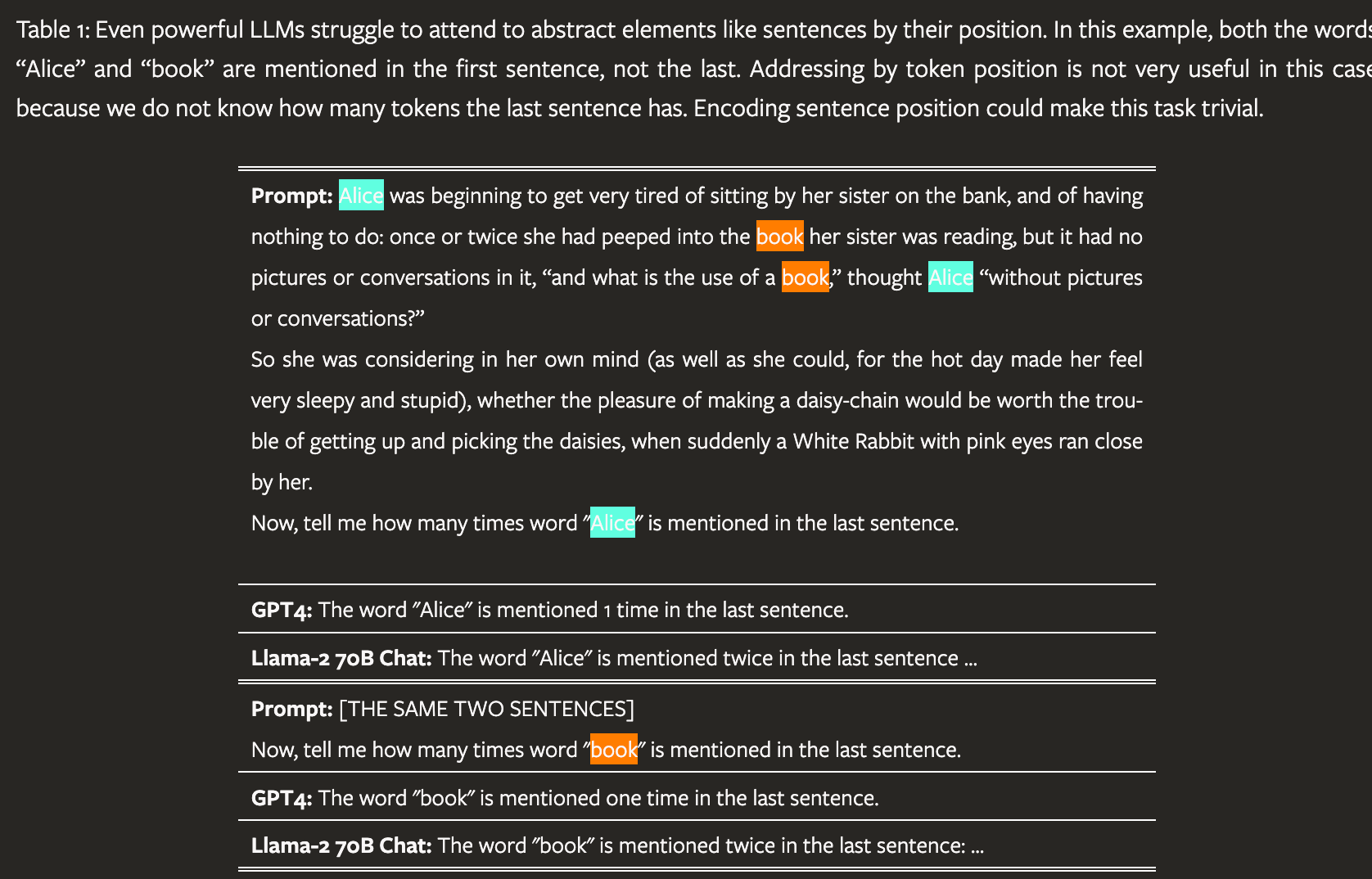
If you remember, we talked about xLSTM couple of weeks ago and mentioned that perplexity of transformers shoots up after contex window. Take a look at the images.

So the problem is, position encodings are static. They don’t adapt to the content. This handicaps the model in tasks like counting, finding position of nth occurance. Also one thing I still can’t fathom about position encodings is, you have a word encoding which carries a meaning. Then you decide to add some random things to some of the features (see RoPE). No wonder the model over fits on positions. Ok enough of my rant
How do you address the aforementioned problem? Simple, just like any other thing in ML, if something handcrafted doesn’t work well, learn it. Yeah you heard it right. Learn it. Add more parameters. But not in any random way. Attention is all you need experimented with learned position encodings but claim that they didn’t find it needful or fruitful. So you have to be more mindful about it. So if you want to do something that is context sensitive, what would you do? The question sounds eerily familiar right? Yes, Attention. You use queries, to query keys and the similarity hopefully will give you enough info to infer something.
Because we already calculate queries and keys for attention, we can simply reuse them for position encodings. Note that authors study different queries and keys but didn’t find it really needful. More specifically, for every position before the current, calculate that context info by dot product of query of this position and key of the previous position, pass through non linearity and sum them up. This acts as a gating mechanism and helps in deciding how much info from the j th token should flow into attention computation for i th token. Notice that due to sigmoid, the max for Pij would be T the total sequence length. And if all the sigmoids are 1, pij would be i-j+1 which is basically relative position encoding.
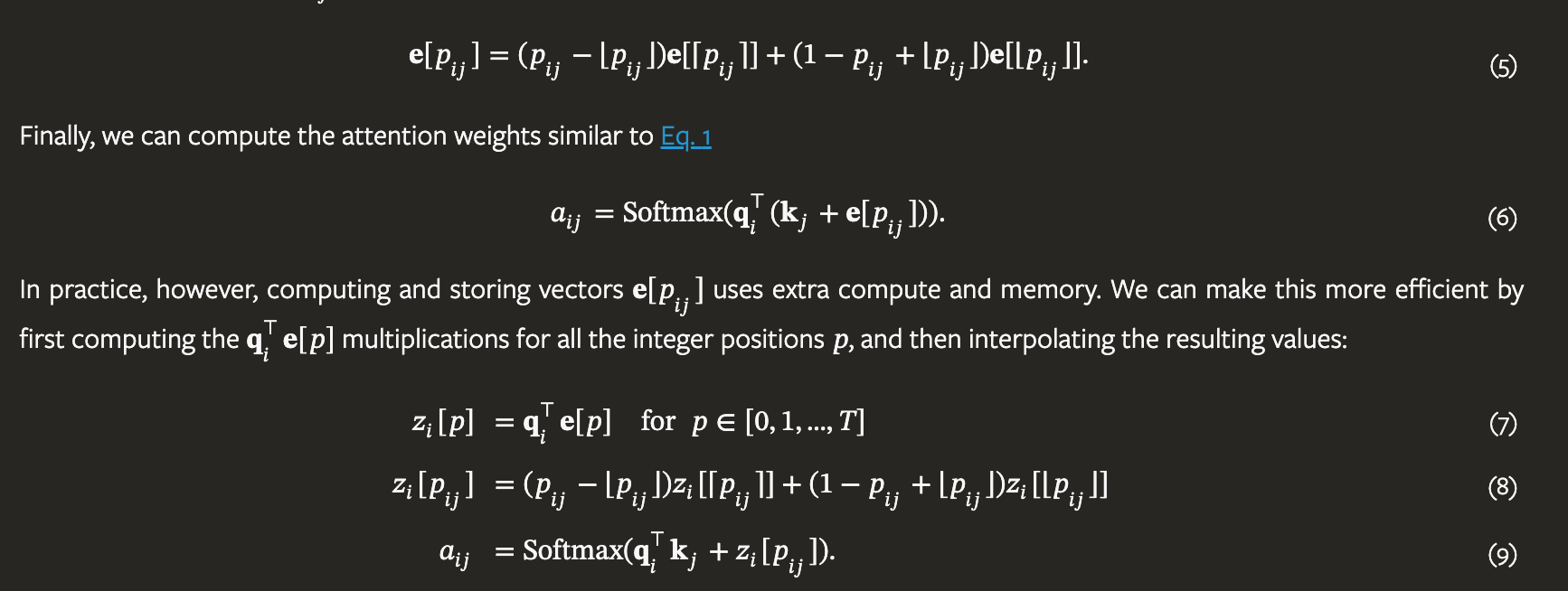
Here, the value of Pij would be a float scalar. This Pij is positon val of j for position i. Now how do you convert this info into a vector to add to the query? Asssume that you had a learnt vector for each position from 0 to seq_len, we can look into that. But we’ve floats, so lets just round off Pij to nearest integers and interpolate between those positions’ encodings. e[pij] is the position encoding you add to query of ith token in case of key of jth token and the equation 5 you see is basically linear interpolation.
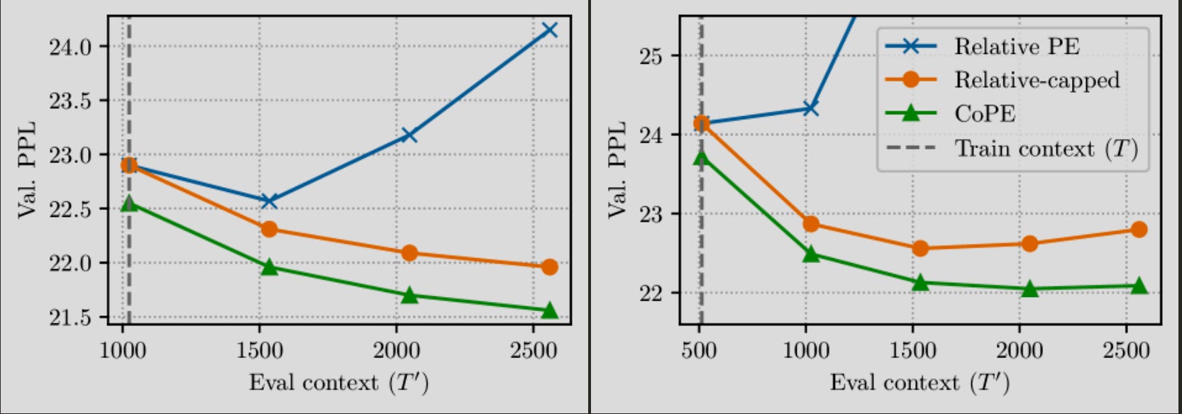
That is pretty much it for the theory, now on to the results. As you see, CoPE generalises to longer contexts (than training) as compared to Relative PE (would be the same for RoPE and Sinusoidal).
In case of say focusing on paragraph, the position attention is focused primarily on nearer tokens (near diagonal is greener) and for focusing on section task, attention is spread out across. Hypothetically, if you want to count the number of sentences, the position-attention would be active at the positions of FullStop(“.”).

They train a GPT2 replica model but with CoPE as position encodings and find the perplexity on train and test data is lesser as compared to the counterparts. They also say that this generalises well to out of distribution data.
The paper explores a new approach at position encodings. But with this, compute would definitely go up a little. Though this looks promising, we don’t know how this effects larger models. The example of Alice and Book mentioned previously, wasn’t attempted to be answered by CoPE, maybe because the model is too small to do that. Is it worth the trade off? If LLMs can now do math with CoPE, I’d say definitely yes. But that would also depend on tokenisation. Until then, we cope with no CoPE :)
Is DPO superior to PPO
The world of Large Language Models (LLMs) research is buzzing with efforts to make these models more in line with human preferences. We often tweak them using methods like Supervised Fine-Tuning (SFT) and Reinforcement Learning from Human Feedback (RLHF). While SFT is generally to teach new knowledge or skill, RLHF is to align the models’ outputs. RLHF has two main flavours: one where we rely on rewards (like a score on a test for humans), and the other where we skip that step and dive straight into training the model's behaviour. Think of RLHF like teaching the model to make decisions. We want it to learn from examples of what is good and what is not, so it gets better at generating responses that we like. Two such popular methods are Proximal Policy Optimisation (PPO) and Direct Preference Optimisation (DPO).
Picture the LLM as a decision-making process ie Πθ(y|x) where represents the model's parameters), where it takes your input (𝑥) and generate a response (𝑦) in an auto-regressive manner. The goal in RLHF, like any other ML training, is to maximise an objective function Jr(Πθ) which combines a reward function r(x, y) and a regularisation term to ensure we don’t deviate from the reference model ref . The constant β is to control this term. The regularisation term in the log you see is trying to minimise the difference in distribution of outputs of reference model wrt to the policy model. This is to ensure that the RLHF-ed model’s outputs don’t deviate too much from SFT model’s outputs to avoid things like reward hacking and hallucinating.
To optimize this objective, let’s consider the two approaches we talked above:
PPO (Proximal Policy Optimization): This reward-based method initially entails training a reward model rΦ using human-labeled data. We show the model pairs, known as preference pairs: one response marked as "win" and the other as "lose", and ask it to pick the better one. Once the reward model is honed, PPO optimizes the policy by maximizing the objective function, minimizing the negative log-likelihood derived from these preferences.
The probability of winning output being likelier than losing one is calculated as follows and the loss is calculated as expectation of negative log liekelihood of diff between
\(p(y_w > y_l | x) = \frac{\exp(r_{\phi}(x,y_w))}{{\exp(r_{\phi}(x,y_w))} + {\exp(r_{\phi}(x,y_l))}} = \sigma(r_{\phi}(x,y_w) - r_{\phi}(x,y_l))\)\(L_R(r_\phi) = -\mathop{\mathbb{E}}_{(x,y_w,y_l) \sim D} [log \space \sigma \space (r_{\phi}(x,y_w)-r_{\phi}(x,y_l))] \)DPO (Direct Preference Optimization): DPO takes a different route. Instead of bothering with a reward model, it directly fine-tunes the policy using preference data. DPO derives a solution that relates the reward r(x,y) to the optimal policy *(y|x). The key insight is that this relationship facilitates re-parameterization of the objective function, ultimately eliminating the need for explicit reward modeling and streamlining the optimization process. A closed form solution is derived for optimization problem.
The loss looks monstrous but doesn’t involve an explicit reward model. The idea is that the language model is itself a reward model (as used by instructgpt for eg)
\(\ell_{\text{DPO}}(\pi_\theta) = -\mathbb{E}{(x, y_w, y_l) \sim \mathcal{D}} \left[\log \sigma\left(\beta\left(\log \frac{\pi\theta(y_w \mid x)}{\pi_{\text{ref}}(y_w \mid x)} - \log \frac{\pi_\theta(y_l \mid x)}{\pi_{\text{ref}}(y_l \mid x)}\right)\right)\right].\)
DPO offers a straightforward alternative to PPO's complex processes (reward model training and policy optimization). By embedding human preferences directly into the training loop, DPO saves computational resources and avoids the challenges of maintaining reward model accuracy. While DPO simplifies reward model training complexities, it faces certain limitations. To demonstrate these, the paper provides theoretical and empirical analysis.

Experiments conducted show that DPO performs poorly when there is a distribution shift between the training data of the base model (Alpaca dataset) and the preference data (SafeRLHF dataset). Mitigating the distribution shift by generating new responses with the fine-tuned model and using a learned reward model for preference labeling (DPO-Iter) achieves comparable safety rates with PPO (Proximal Policy Optimization), another method. However, DPO-Iter obtains lower helpfulness rewards compared to PPO.
So the conclusion is, if your task is challenging, PPO offers better results. If you need to improve on two separate things, DPO is probably the better alternative. If you don’t have the compute to train for Reward model, DPO is the only choice then. DPO avoids suffering from reward hacking. DPO can produce wider variety of solutions (including the PPO one) but might also lead to unwanted unexpected solutions. The best part about DPO is as long as you have different data, you can apply it multiple times without relying on other model.
S3D: Self Speculative Decoding Scheme
Speculative decoding is an innovative method to speed up text generation in large language models (LLMs) without sacrificing output quality. This technique is gaining popularity for its efficiency. Here’s how it works.
Drafting Phase: The model quickly generates a sequence of potential next words or tokens, prioritizing speed over accuracy.
Verification Phase: The model then thoroughly checks these drafted tokens with a full forward pass, ensuring their accuracy.
The initial rapid guesses are often correct or close enough, allowing the verification phase to efficiently confirm them. The time saved during the drafting phase offsets the detailed verification time, resulting in a faster overall generation process.
Since blockwise parallel decoding was proposed, predicting the next k tokens simultaneously has proven effective. This method requires adding k feed-forward decoder layers from the last encoder state. Medusa enhanced this with Medusa heads and tree attention, fine-tuning only the new heads. This is very much similar to Multi Token Prediction by Meta we discussed earlier and there too we talked about how it can help Speculative decoding…
SpecDec uses an independent encoder-decoder model with distinct attention queries for each token, unlike Block-wise Decoding's shared query, but requires full model fine-tuning.
Multi-token prediction can also be done auto-regressively (Hydra, EAGLE) predicting the next token in steps based on previous drafts. To reduce overhead, this process must be efficient yet effective. EAGLE achieves this by combining the target model’s high-level features with the next tokens' embeddings for regression via an extra Transformer decoder layer. Unlike Medusa, which predicts tokens at various offsets solely using the second-top layer's features, EAGLE incorporates the next token's embedding, improving its handling of sampling randomness.
The proposed S3D uses a draft model and adapts Masked Language Modeling to predict multiple future tokens simultaneously. For an input sequence t1, t2, .., ti, the draft model predicts ti+1, ..ti+γ based on the current sequence and special mask tokens (<M>):
The draft model, Mq, relies on the hidden states from the full target model, to maintain accuracy. Specifically, the hidden state at the current layer is a transformation function of the previous layer's hidden states and the positional encodings up to position i.

When generating tokens simultaneously (at positions j = i + 1, i + 2, ..., i + γ)
the method only processes the initial (1 through m) and top layers (n through L) of
the target model, skipping the middle layers. Hidden states are computed as usual
for the non-skipping layers, and the hidden state at layer (n − 1) is set directly to
the hidden state at layer m, where l′ indicates all the non-skipped layers. This ensures robust foundational representations before skipping to higher layers.
In one of our previous blog posts outlining Mixture of Depths, we mentioned how the hidden states of different layers in a transformer are very closely related thanks to the Residual connections. The cosine similarity between activations of layers seperated by 10 layers can be as high as 0.85. So one in theory can pretty much just skip these layers with minimal loss in accuracy.
S3D’s training uses a loss function, LS3D, that accounts for the negative log-
likelihood of predicting the correct token at j+1 given the context up to j. The
skipped layers are frozen to preserve the target model’s learned distribution.
Here D is the decoding set which includes the positions {i, i + 1, ..., i + γ − 1}. Additionally, masked tokens are randomly assigned and batch processing maximises efficiency and leverages Transformer parallelism.
Predicting Speedup: The target ratio β represents the portion of the target
model’s parameters used by the draft model, influencing the acceptance rate α.
The authors hypothesised a function to estimate α based on β and model size
parameter U . This function aligns with empirical results.
For multi-token predictions, the acceptance rate decreases with each subsequent
token, and the expected number of newly generated tokens τ(γ, β) is calculated
using a sum of products involving the acceptance rates. For every token 1 to γ+1, we take the expected acceptance. Like for 1 token acceptance, n=1 and the product denotes the possibility of accepting 1 token and rejecting n-1, for n=k tokens, the product term is acceptance of k-1 tokens Παk(β) and rejecting the k+1 th = 1-αk(β)
When the number of drafting tokens is not significant (something like drafting 4 tokens say, which commonly happens on low-end devices), it is reasonable to assume the time cost for a full-model forward pass (passing those 4 tokens for verification through the full model) to be a constant C (which is generally around the order of time taken for one token forward pass). We also assume there is a fixed overhead (processing n_draft tokens takes little more than just 1 token, so) H0 for each iteration, proportionally to C, i.e., H0 = δ.C. The Improvement Factor for self-speculative decoding (assuming that the forward time for a partial model scales linearly with the number of its parameters aka passing through 10 layers take 1/4th the time of 40 layers). Denominator is 1 for full pass + δ overhead + β for partial model pass
The explanation here is, if you accept X tokens and it takes the time equivalent to generating Y tokens, the improvement is X/Y. So the numerator Expected number of tokens denotes how many tokens we generate on average. The denominator denotes how much time (as a ratio wrt generating 1 token as explained above) it takes for that. The overall equation is the Improvement Factor.

S3D demonstrates high speed and effectiveness across various GPUs compared to CLLM, maintaining baseline effectiveness and surpassing models requiring target model training. Despite closely matching EAGLE in speed and slightly underperforming CLLM, S3D excels in memory efficiency, outperforming EAGLE while using less VRAM. It operates within a 16 GiB VRAM limit in half-precision and outperforms quantised EAGLE by up to 3.9 times, emphasising memory efficiency's importance. Unlike CLLM's training objectives, which may degrade effectiveness, S3D preserves effectiveness scores robustly while achieving optimal speed-memory ratios.
Speculative decoding offers a unique way to speed up LLM inference without sacrificing on quality if you have a good draft model. But the biggest constraint would be memory. Loading and inferencing two models is not an easy task. Self speculative decoding offers an elegant way to tackle that. And S3D is a member of that family. Now instead of statically removing layers, if we follow the footsteps of Mixture of Depths, we can probably improve performance even further.
 | A guest post by
|
 | A guest post by
|