


AI Unplugged 16: Llama 3, AIMO winners, Segment Anything Model 2, LazyLLM
Insights over Information


Table of Contents
Llama 3 Herd of Models
AIMO: Findings from the winners
SAM 2: Segment Anything Model 2
LazyLLM
Llama 3 Herd of Models
We have already talked about Llama 3 family of models. Meta released the paper about the same. We will. go over any new piece of information. There is also new model with 405 billion parameters. All in all the series is called Lama 3.1.
Just like the smaller models, the 405 billion parameter model is also trained on 15.6 trillion tokens on a cluster of 16,000 H100 GPUs They also used models like Roberta (trained on llama2 predictions) to filter out and create a high-quality data set.

If you observe closely, the learning rate decreases with increase in model size. It is common knowledge to decrease learning rate with increase in batch size. And that is probably what happened too. It is mentioned that lower batch sizes were used initially to kick off the learning and it is increased over time. 4M tokens batch size at 4k context till 252M tokens aka 63 steps (idk why they stopped just before hitting 64 steps though). Then bumping up to 8k sized tokens totalling to 8M till a total of 2.87T tokens aka for ~360 steps.
For Alignment, along with chosen and rejected samples, there is also an edited sample which is an improvement over the chosen sample. But instead of having 3 examples with scores for each, input prompt with three responses into a single example. DPO is the chosen alignment policy. Along with that, a negative log likelihood (NLL) is used as stabilising term. Also, for special formatting tokens (which denote turns like <s> or [INST] ), are ignored from loss calculation. This is because the same tokens appear in all chosen, rejected and edited samples. This might confuse the reward model. Very much like ORPO (Odds Ratio Preference Optimisation)
The context window is then gradually increased in six stages to 128k for a total of 800B tokens. They use a cosine learning rate schedule with decay to 1/10th of the original learning rate. The first few steps are for linear warmup where you slowly inc learning rate from 0 to max learning rate. The last part is annealing where the learning rate is dropped till 0 over 40M tokens. Annealing on High Quality data at last is said to improve model quality. This was also noted by MiniCPM 2.0 and other works.
For DPO, training only on short context data, doesn’t negatively impact Long Context performance given that SFT model is already good at long context. DPO only steers the model response style primarily.
Essentially, you always always start with small context length, let the model get familiar with data and language, then slowly increase the context window. A kid doesn’t learn to remember page long contexts directly. One has to teach them to learn one sentence at a time, then one paragraph and at last, whole page or chapter.
Another interesting is the new scaling laws. This time around we try to correlate the compute flops with negative log likelihood on downstream task instead of next token prediction loss aka something like validation loss. There are also relations between the said loss and the model on those tasks. Hence, optimal params (N) for a given compute budget (C) given compute budget is given by the relation.
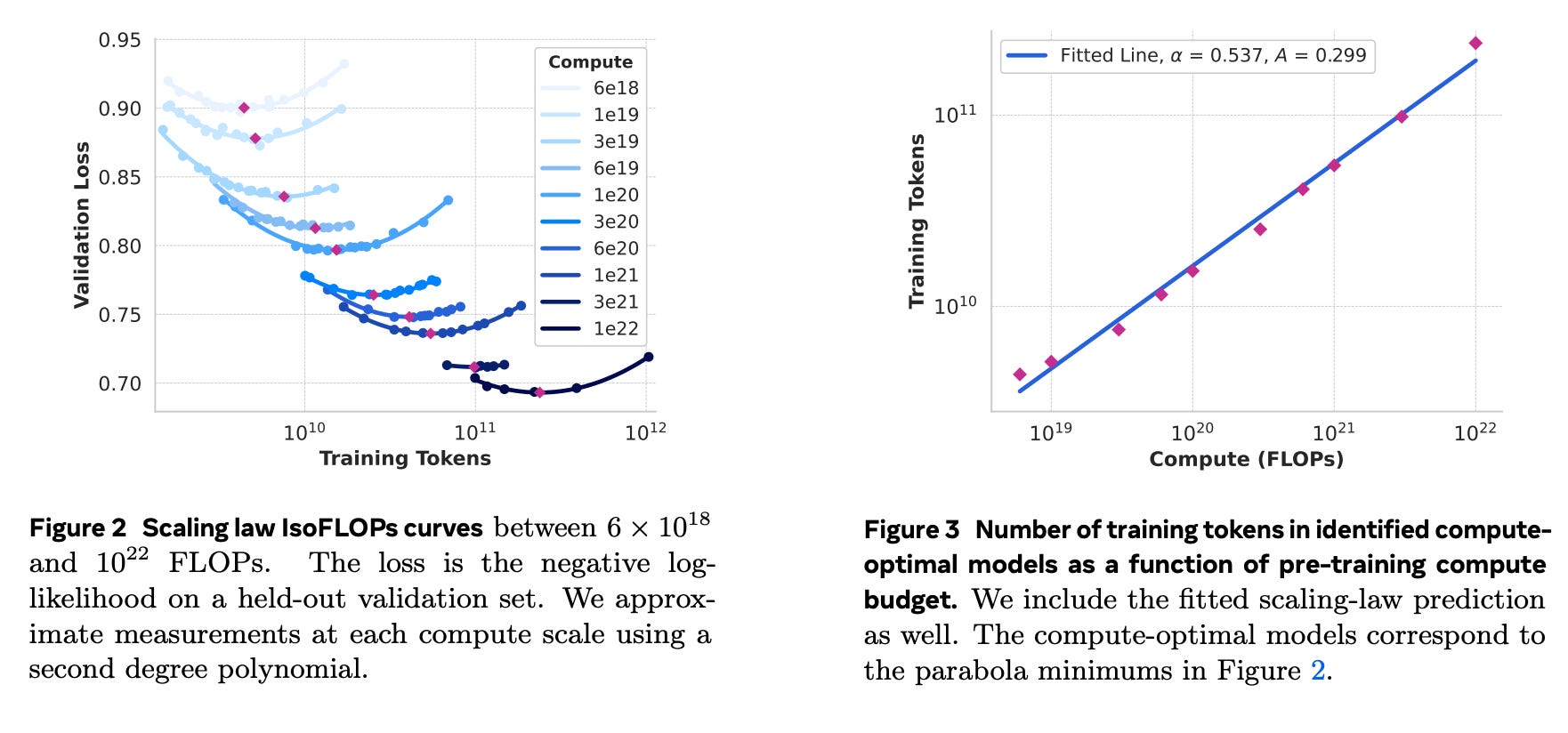
You also see the validation laws curves looking like a parabola. this means that there is a model with the optimal performance, anything bigger or smaller will lead to either under fitting or over fitting. At the same time, the curves get flatter as the compute increases, which means that the models get more and more robust as the compute or the model size increases.

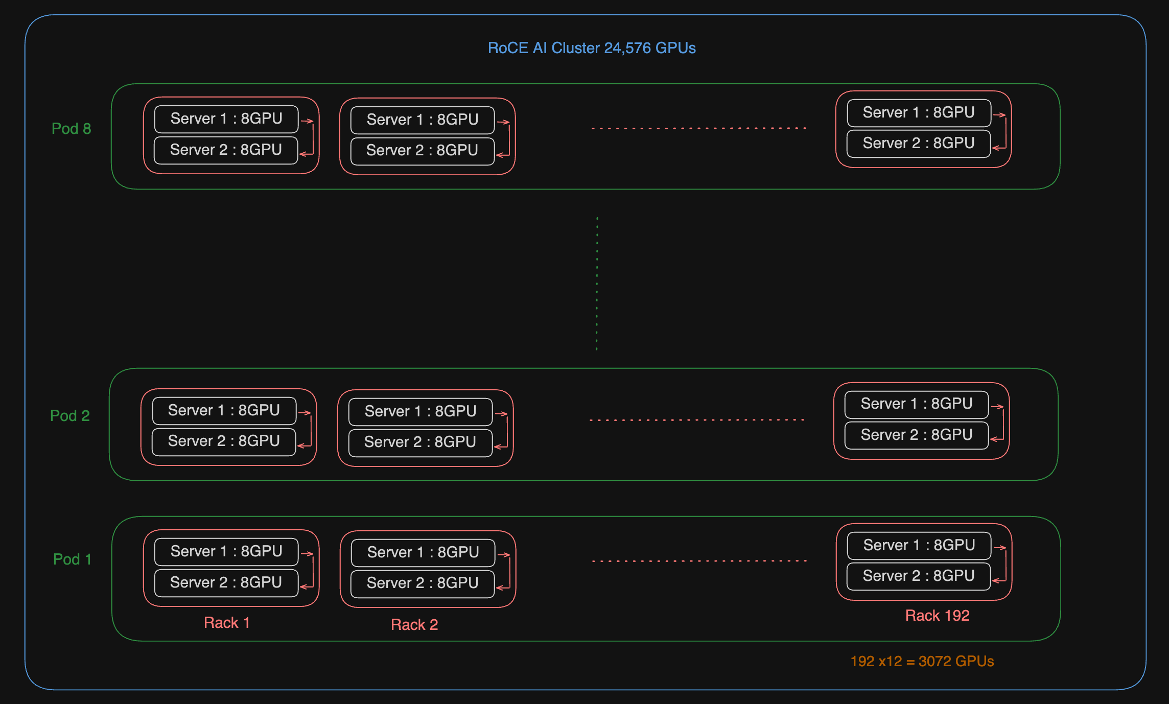
There is also info about what causes the training runs to fail at such a big scale. Surprise surprise, it is faulty GPUs which cause ~30% of failures. And there are a lot of parallelism in place to speed up things. From Tensor Parallelism to Pipeline parallelism. With that, they achieve an MFU (Model Flops Utilisation) of 40% on H100. This is decent GPU utilisation.
Coming to the data, as said earlier, Roberta and DistilBERT are used to filter out data as first step. Then to counteract over apologetic behaviour that we see in models like ChatGPT, samples containing the phrase “I apologise” and “I’m sorry” are balanced out. To further filter out data, the scores from the reward models are used as one feature and scores from LlaMA 3 8B model (prompt based scoring) and those that score high (top 25%) are used for training.
Along with that, LlaMA 3 70B is prompted to calculate the difficulty of a given sample. The product of difficulty score and quality score is used as a proxy to filter data.
The models are then trained on 1T tokens of (>85%) code. For reference, llama 1 family of models are trained on 1T tokens in total. How far have we come in 1y lol. Later, 2.7M synthetic data samples are generated for SFT on code. This only helps when model generating the code is bigger (aka better) than the trainee model. It makes us think, can we use Distillation (like Gemma 2 family) instead of training on hard model generated labels of code? I think so, but this isn’t explored in llama3.
To counter the fact that most of the code is generally Python or C++ with other languages having very little contribution, the code in major languages is translated to those unused languages.
Along with code and multilingual data, tool usage has been a point of focus for llama3 family. Interestingly, they are trained to use Brave API instead of any other search engines like Google or Bing. Brave has an assistant called Leo which uses LlaMa 2 70B. So the likes of a partnership ig. Apart from search as tool, the other tools used are Python Interpreter and WolframAlpha for math. Given the model’s abilities to perform in context learning, the models can perform tool usage with in context learning.

For multimodal learning, the dataset is filtered based on CLIP score. Deduplication of data is also done to improve model training and quality. The image encoder is trained on 6B image-text pairs (welp, owning Instagram helps ig). The training is done at a batch size of 16384 and initial learning rate of 1e-4. For videos, 16 frames are sampled from the whole video, uniformly in time. The speech encoder is trained on 15M hours of audio. Maximum length of each audio is 60 sec.
All in all, a detailed paper about choices and decisions is a welcome. In a time frame where model releases have turned into benchmark scorings, this is a welcome move for the advancement of the field. Key take aways from the LlaMA 3 paper are
Annealing with High quality data
Synthetic data generation
Progressive increase in batch size and context length
It’d have been great had Knowledge Distillation ben given a try like Gemma family.
AIMO: NumniaMath and CMU-Math
AIMO is the AI version for IMO. It has been recently concluded and provides us with a wonderful opportunity to reflect on the winning ways. If AI can solve AIMO aka IMO, its a great step in the direction of advancement of models. From not being able to solve basic addition to solving probably world’s toughest exam. For AIMO, the competition featured 2 sets of 25 problems each. Competitors can submit fine tunes of open weight models. The model has to run on 2xT4 GPUs or P100 with 9 hours to solve the questions.
NuminaMath has won the competition while CMU Math were the runners up in the competition. We’d start with NuminaMath. The model is based off of DeepSeek Math 7B Base.

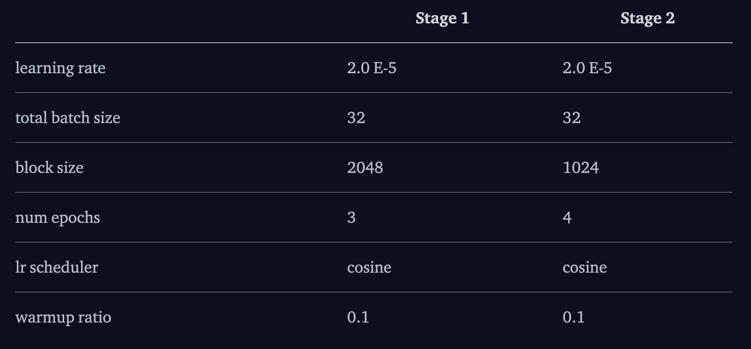
Fine tuning, inspired from MuMath Code is done in two phases. In the first phase, we use large dataset with Chain of Thought solutions to given problems. The second phase consists of synthetic data of tool integrated reasoning. The dataset is generated by GPT-4. Here’s a look at hyper parameters used for both phases. Because Stage 1 uses CoT, the block size is larger. The second stage is key as it involves tool usage. With just stage 1, the model only gets 8/50 solutions correct.
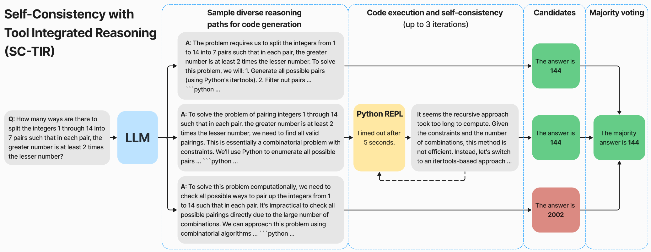
They generate data from multiple sources like solutions in PDFs of various olympiads. GPT4 is prompted to generate Tool Usage solutions and those with incorrect final answer are rejected. Self Consistency Chain of Thought is employed as is evident from the image below.
To fit within the GPU constraints, the model is quantised to int8. Because the public test set is only of 50 problems, to avoid any overfitting, internal validation sets are used. Such data is generated from questions of other olympiads like AIME and AMC
Numina also experimented with KTO. The advantage with KTO over other methods like PPO or DPO is that you don’t need pairs of samples. All you need is, given a sample, information of whether it is a positive one or a negative one. This eases out a lot of data labelling/generation troubles and the problems of dealing with random sample as negative for alignment. Given the outputs of SFT model, label them as correct if the final output is correct and wrong otherwise. This produces a model which is slightly better than pure SFT. Another interesting thing is, the same training recipe, when applied to bigger models like InternLM-20B, CodeLlaMA-33B or Mixtral-8x7B couldn’t outperform DeepSeek Math 7B because the latter has been explicitly trained on math data and also those models would be very slow to infer on T4 GPUs.
Now onto the runners up, the CMU-Math model. Right off the bat, there’s a major change from NuminaMath. Instead of relying on a single model for submission, CMU-Math makes use of two models. The two models are dubbed Policy model, which generates candidate solutions and Reward model which rates the solutions.
The models are based off of DeepSeek-Math-7B-RL unlike Numina which uses DeepSeek Math 7B base. But like Numina, CMU also uses programatic approach to solve problems. After all, plain text is prone to hallucinations and one miscalculation somewhere can lead to drastically different outputs. It also provides the flexibility to utilise already available functions (like matrix inverse) with ease.

Just like Numina, CMU also uses AIMC and AMC and filter out only integer answer questions. This resulted in 2600 sample dataset. They are then fed to GPT-4o and DeepSeek Coder V2 to scale the dataset to a total of 41,160. They have open sourced the dataset here. On the same data, the DeepSeek model is trained for 3 epochs with a learning rate of 2e-5 just like Numina. Interestingly, they compare the data generation costs to that of Numina and claim that Numina would’ve spent ~$100,000 while they only spent $1000 owing to a 20x larger dataset size.
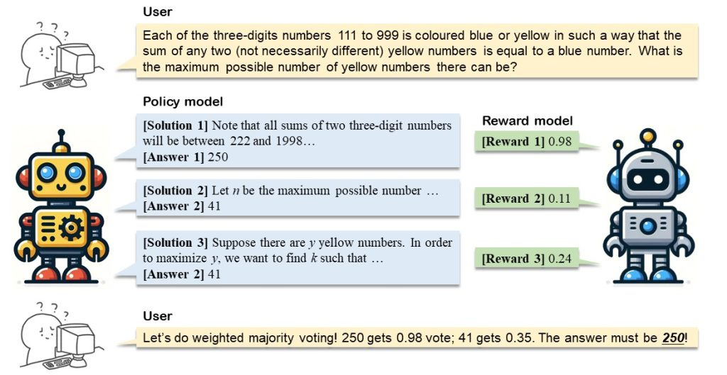
One interesting observation is that the policy model in itself, prone to hallucinations, generated wrong answers more number of times over the correct ones for some (2/10) training samples. So basically, the models are hallucinating. To counteract this, the Reward model is introduced. After all, judging something is easier than generating. This is the exact reasons why GANs produced amazing results. To generate data with both correct and incorrect samples, they needed a model that can do both.
So they turned to interpolating weights of DeepSeek Math 7B base and RL variants. The former generated wrong solutions while the latter generated correct ones. Controlling the interpolation ratios, one can hypothetically control the problem solving strength of resulting model. Hence generating answers that are wrong at different depths of solution. Creative approach to a seemingly blocking problem :). In fact, because we’re training for 3 epochs, one can utilise the checkpoints of 1st and 2nd epoch to further generate unique solutions (both wrong and correct).
SAM 2: Segment Anything in Images and Videos
The Segment Anything Model (SAM) is designed for promptable image segmentation, made up of three key parts: an image encoder, a flexible prompt encoder, and a lightweight mask decoder. First up, the image encoder. It uses a Vision Transformer (ViT) pre-trained with a masked autoencoder (MAE). This lets it handle high-res images smoothly, transforming them into a 256-channel embedding that's both scalable and efficient. Next, we have the prompt encoder, which deals with different types of prompts.
Input prompts are usually mask images, coordinates (points) or bound boxes. For prompts representing sparse objects such as points and boxes, typically represented by a tuple of 3-4 numbers corresponding to the coordinates of points, positional encodings and learned embeddings are used. For prompts corresponding to dense objects like masks or tracking a single object, it downscales the input image using convolution and merges them with the image embedding. Finally, the mask decoder blends image and prompt embeddings using a modified Transformer decoder that employs self- and cross-attention. This process updates the embeddings, upscales them with transposed convolutions, and passes them through a small MLP to create the final segmentation mask.
SAM2 builds on SAM to enable video segmentation. The traditional ViT image encoder is replaced with Hiera, a hierarchical version inspired by ResNet where the images are processed at different resolution scales. It handles fewer features in the early layers and lowers the spatial resolution in the later layers. This hierarchical setup incorporates high-res info through a feature pyramid network with positional embeddings spread across windows. For dealing with time (because we're talking videos now), SAM2 introduces memory attention module. This conditions the features of the current frame based on the past frames' features, predictions, and new prompts, all using a series of transformer blocks. Each block does self-attention followed by cross-attention to memories stored in a memory bank.

For temporal processing, SAM2 introduces a memory attention mechanism. It conditions the features of the current frame on past frame features, predictions, and new prompts using a series of transformer blocks. Each block performs self-attention followed by cross-attention to memories stored in a memory bank. The mask decoder gets a boost with skip connections from the hierarchical image encoder and uses self- and cross-attention to update and upscale embeddings into segmentation masks. It even has an extra head to predict if the object in question is present in the frame (occlusion scenarios).
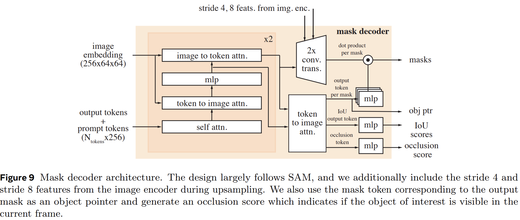
The memory encoder generates memories by downsampling the output mask and fusing it with the unconditioned frame embedding using lightweight convolutions. The memory bank keeps a FIFO queue of recent frames' memories and prompted frames' memories, along with object pointers for high-level semantic info. It also reuses image embeddings from the Hiera encoder and projects memory features to a dimension of 64, with object pointers split into 64-dimension tokens for cross-attention.
SAM 2 is compared against existing state-of-the-art methods using standard protocols. SAM 2 significantly outperformed previous methods in both accuracy and inference speed (FPS). Larger image encoders give a noticeable accuracy bump. On the SA-V val and test sets, which test performance on open-world segments of any object class, SAM2 shines, showing it can "segment anything in videos." Notable improvements were also observed in the long-term video object segmentation benchmark (LVOS).

A bunch of ablation studies were performed to fine-tune SAM2, checking it out on the MOSE development set, SA-V val, and across 9 zero-shot video datasets. Higher input resolution boosts both image and video tasks. Training with more frames improved video benchmarks, settling on 8 frames for a good speed-accuracy balance. More memory size generally helped, with 6 past frames being the sweet spot. Using 2D-RoPE in memory attention was a win. Adding a GRU before the memory bank didn’t help much. But cross-attending to object pointers from the mask decoder output gave a big performance boost on the SA-V val dataset and LVOSv2 benchmark.
LazyLLM: Dynamic Token Pruning for Efficient Long Context LLM Inference
Standard prompt-based inference with large language models (LLMs) involves two main steps: prefilling and decoding. During prefilling, the model takes the prompt - a sequence of tokens - and processes each one to build the key-value (KV) cache. This stage ends with predicting the first token after the prompt, and the time it takes is known as "time-to-first-token" (TTFT). After this, the decoding stage kicks in, where the model uses the KV cache to predict the next tokens one by one until the output is complete. The KV cache is super handy because it cuts down on the computation needed during decoding since the model doesn’t have to reprocess the entire prompt.
Prefilling can be a bit slow, especially for long prompts. This stage can take a lot longer than the actual decoding, making up a big chunk of the total time to generate text. For instance, on average, TTFT can be 21 times longer than each decoding step and makes up about 23% of the total generation time on the LongBench benchmark, which involves prompts of around 3376 tokens and outputs of 68 tokens.
LazyLLM only computes the KV cache for tokens that are crucial for predicting the next token, pushing off the rest until they're actually needed. This method uses attention scores from earlier transformer layers to figure out which tokens are important and progressively prunes less important ones. But it doesn’t completely ignore them; they can be brought back if necessary. This selective pruning keeps performance high while cutting down on computational load.
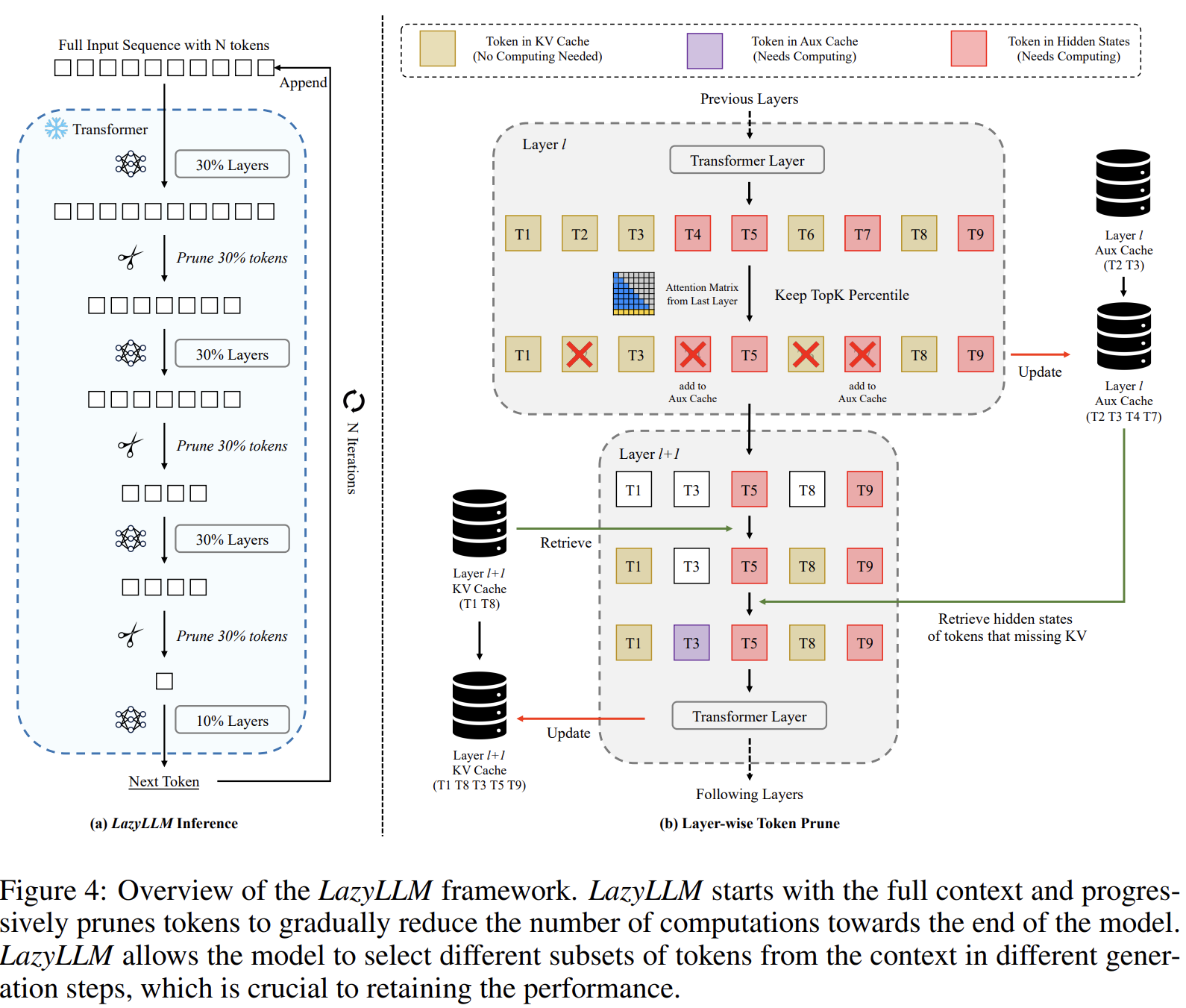
The process of progressive token pruning involves evaluating the importance of each token based on attention scores from the transformer layers. Less important tokens are pruned through the layers using a top-k percentile selection strategy, which means tokens with lower confidence scores get pruned if their scores fall below a certain threshold. Performance varies depending on where pruning happens and how many tokens are pruned. Pruning in later transformer layers tends to perform better, suggesting those layers are less sensitive to token pruning. To balance speed and accuracy, LazyLLM progressively prunes tokens, keeping more in the earlier layers and reducing them towards the end. Additionally, LazyLLM also introduces an auxiliary cache (Aux Cache) to store hidden states of pruned tokens. The Aux Cache ensures that even if tokens are pruned at one stage, their hidden states can be efficiently retrieved for future use, maintaining computational efficiency.

LazyLLM was tested with two large language models, Llama 2 7B and XGen 7B, on LongBench, which covers a variety of tasks including question answering, summarization, few-shot learning, synthetic tasks, and code completion. LazyLLM achieved better TTFT speedup with minimal accuracy loss across these tasks, showcasing its efficiency. Increasing the number of pruning layers and the amount of pruning generally improves TTFT speedup by reducing the tokens processed. Pruning tokens earlier saves more computation for later layers, but too much pruning can hurt performance. Both Llama 2 and XGen showed similar trends: performance dipped with fewer tokens kept at the same layer, and pruning later layers performed better than earlier layers. In a nutshell, LazyLLM reduces the computational load by pruning tokens progressively, particularly in attention layers where costs grow quadratically, ensuring a faster and efficient generation process without sacrificing much accuracy.
 | A guest post by
|
 | A guest post by
|