AIUnplugged 15: Gemma 2, Flash Attention 3, QGaLoRE, MathΣtral and Codestral Mamba
Insights over Information
Table of Contents:
Flash Attention 3
QGaLoRE
MathΣtral and CodeStral mamba
Gemma 2
Yeah, I know its been a while since Gemma 2 was out. Unfortunately I myself didn’t have time to look at things. But I didn’t want to let it go unexplored. So here we are. Gemma was first released in Feb 2024. It came in two size variants. 2B and 7B. They were reportedly better than llama 2 family of models. But since then, a lot has changed. LlaMa 3 came out, Qwen 2 came out, MiniCPM 2 etc etc etc. So in this fast paced AI landscape, the time between iterations is mere months. Now here we are with the successor Gemma2.
It was first announced at Google I/O and the weights were released recently. With this, they release an attached paper which has some really cool insights.
First, lets start with what changed. There are three size variants now, 2.6B 9B and 27B. Let us compare them, shall we? We look at gemma-7b vs gemma-2-9b configs. One immediate change is the architecture shape. The hidden_size increased from 3072 to 3584. This controls how much information flows between layers. Another change is intermediate_size. This is to what size the hidden vectors are projected onto in the MLP. Realistically speaking, if you have a 3584 dimension vector, even if you project it to any higher dimension, it won’t add any new information. So there shouldn’t be much difference in doing this.
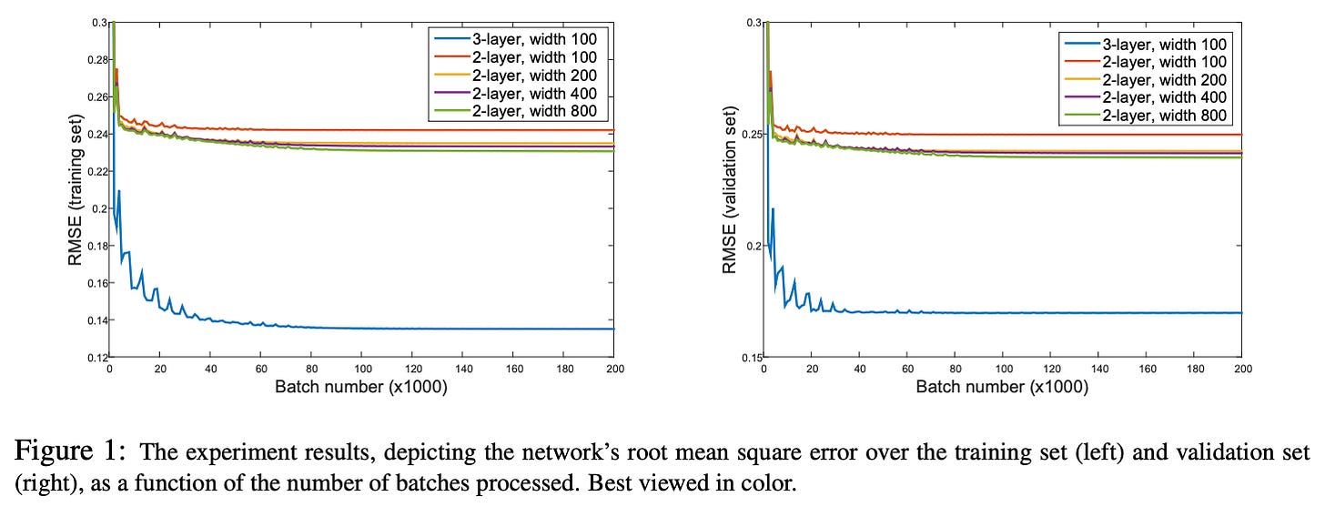
One change that effects performance for the better is num_hidden_layers. This increases the depth of the network. They briefly mention the difference. Deeper network outperforms wider one.
This goes in line with previous research works that show deeper networks are better than wider counterparts.
If you observe the architecture difference image above, the lines 7 and 11 in the right half introduce new variables. attn_logit_softcapping and final_logit_softcapping. This basically artificially clips the logits to the said values. The tanh function clips the values between (-1,1) and then the final multiplication scales that to the said value.
Another change is, the num_attention_heads and num_kv_heads differ in the new config. This means Gemma 2 is using GQA. GQA uses only a portion of key and values compared to queries. This is more efficient than Multi Head Attention.
They also implement layernorm both before and after MLP layers. This is said to improve stability. The said norm is RMSNorm like llama. And every alternate layer, they switch from SWA with local attention on 4096 tokens to Global Attention on 8192 tokens. Infact, their ablation study shows that even if we decrease the local attention window width to 1024, there is very little hit to perplexity
The 9B and 27B models are trained on 9 trillion tokens while 2.6B model is trained on 2T tokens. The most interesting part of the paper is they use distillation to train the smaller 9B and 2.6B models. For the unaware, distillation is where you try to mimic a teacher’s (generally bigger model) output rather than ground truth. This way, the final output is more continuous and hence can lead to better/faster training. I’m curious what 7B model they are referring to here. There seems to be no info about it. Maybe gemma 7B, maybe some other 7B model lol. Also, Gemma models on the huggingface hub are in FP32 so be careful about your disk space :)
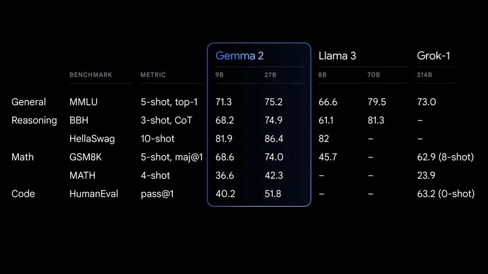
Coming to results, the models, especially 27B is on par with models much larger than its size. LlaMA 3 does outperform gemma 2 27B though. The 27B model ranks at 12th on the LMSys chatbot arena leaderboard which places it a few steps above llama 3 70B. Pretty impressive. The story is the same even on Coding, Instruction following and Multi Turn tasks. The 9B-it model is among the top 20.
Gemma has also gained a lot of love from the community as one of the best models in its size class. People also noted that it is better than LlaMA3-8B especially for multilingual tasks. 9B might be a little too much to run on 16GB GPU at 16bit precision. But one can always use 27B at 4bit which approximately consumes 20GB VRAM. There are also SPPO trained variants of the same which apparently improve the model quite significantly. Also I’m a big fan of ablation studies which tend to test out how much impact each change causes. This is very helpful if you’re trying to build something of your own.
Flash Attention 3
Flash Attention has been an incredible breakthrough in the world of LLMs. It pushed the boundaries of how much GPU utilisation can be achieved if you plan your math accordingly. The whole idea behind flash attention is very very simple. The compute capacity increase of GPUs is outpacing the memory capacity and bandwidth increase. So a lot of training time is spent unnecessarily moving data between GPUs DRAM and SRAM ( something like CPU RAM and cache). It is common knowledge that if you increase cache hit rate, your performance sky rockets.
Original Flash Attention could achieve a speed up of 7.6x. So what changed in matrix multiplication? Well simple, instead of repeatedly copying items from DRAM to SRAM, copy it smartly. I mean, if you copy something to SRAM, make sure you do all the computations that involve the said block of values then and there, thus reducing the transfers per block.
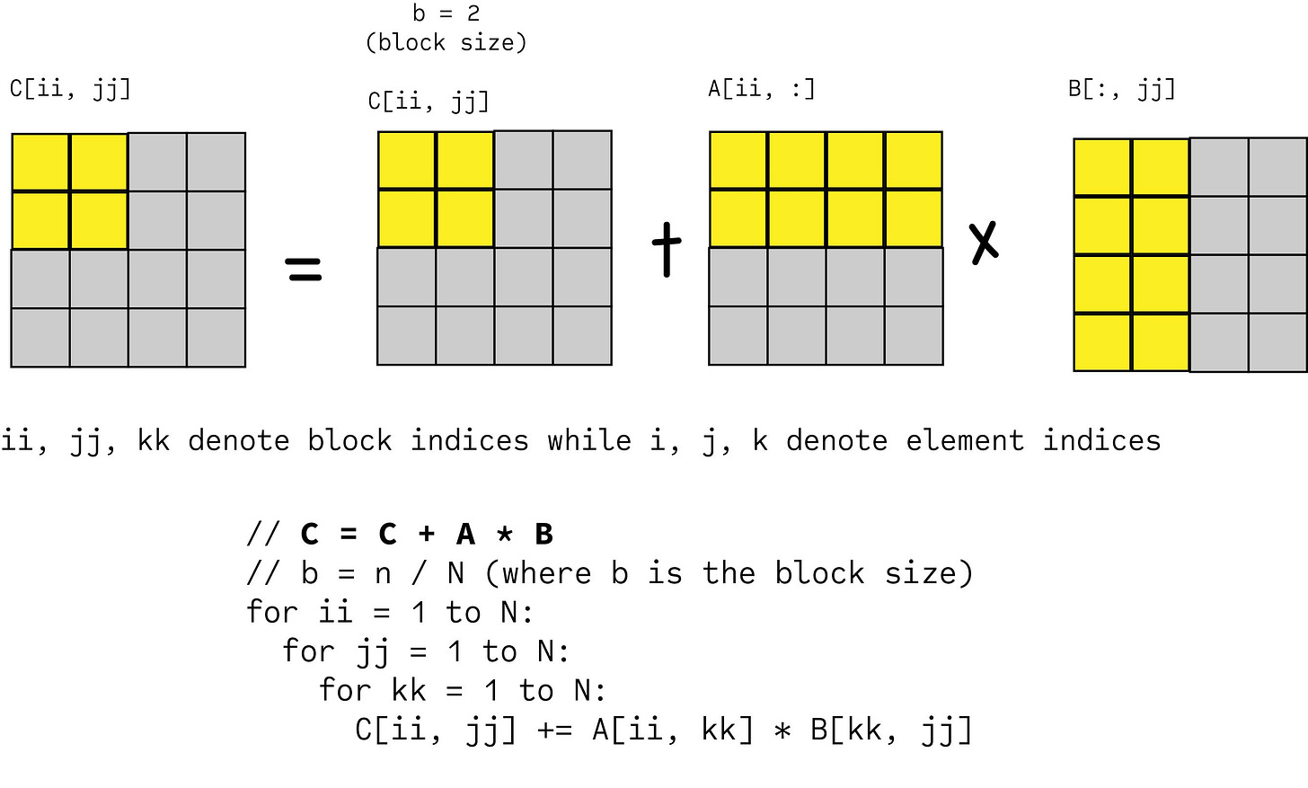
Matrices in deep learning are big. For example, for a small model like llama 2, the attention matrices are 4096x4096. At 16 bit precision (FP16/BF16), this itself is 32MB which is 1.5x larger than the SRAM capacity of data centre level A100 GPU. So multiplication of matrices is generally done in blocks. Each block is treated like a small matrix and the multiplication is carried forward.
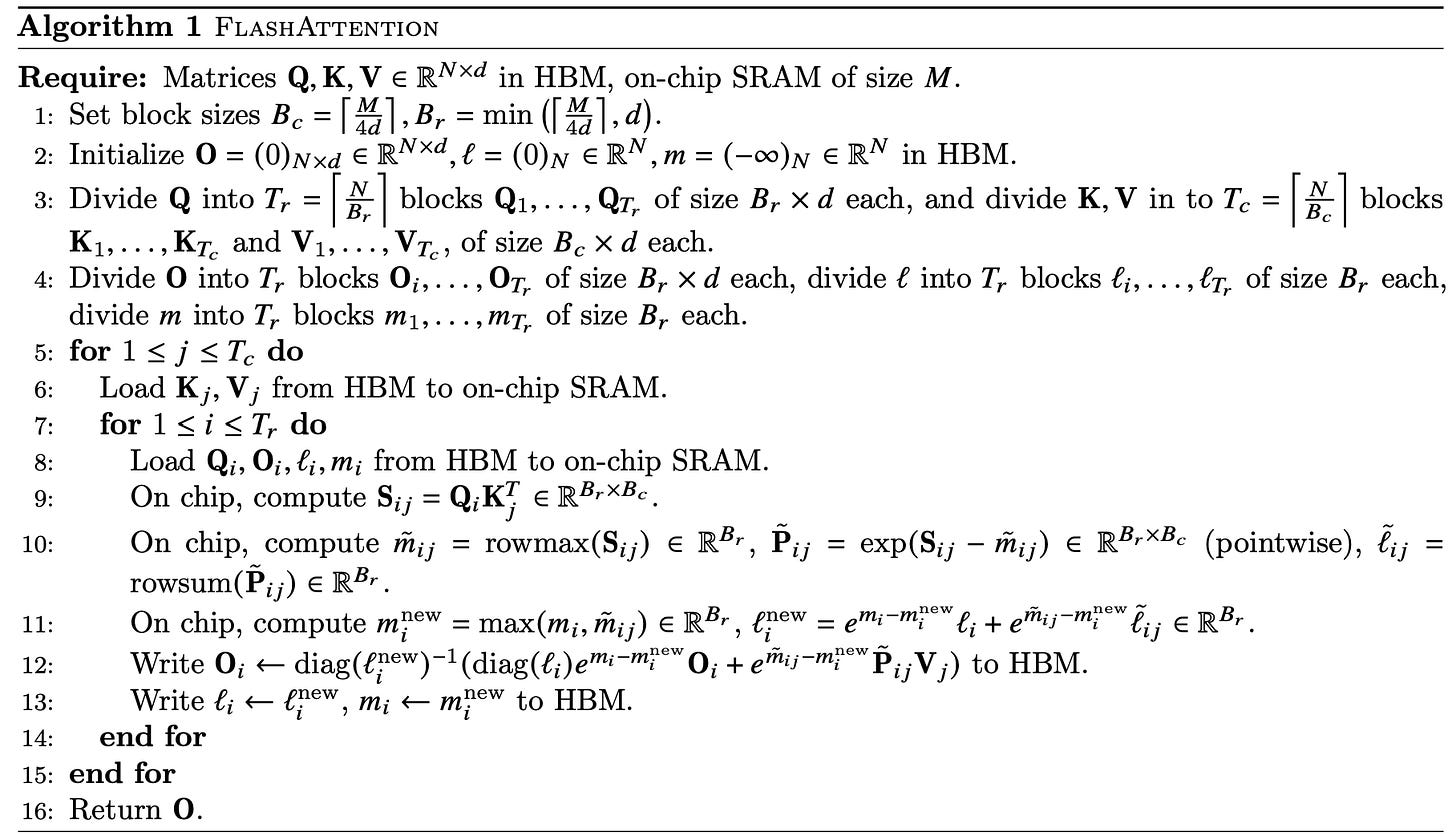
Flash Attention does this very thing but in a smart way. First we need to understand how many matrices (and of what size) we can fit in the SRAM at once. Depending on that we plan our computation. We need to store Query, Key, Value and Output in the SRAM. So we divide the SRAM size by 4 to given equal space to each of the said components. And then divide the original matrices across the sequence length to fit it in. Note that you might need to have a little buffer to store things like m and l. They also use the registers to store some of these values. So all in all, dividing by 4 approximately is the way to go.
Now another important thing is the softmax operation. GPUs have a lot of capacity for matrix multiplications but comparatively very less for non matmuls. As an example, the A100 GPU has a max theoretical throughput of 312 TFLOPs/s of FP16/BF16 matmul, but only 19.5 TFLOPs/s of non-matmul FP32. That is a 15x difference. You have to somehow parallelise the softmax which generally is sequential.
As for why this is true, you can look at the full proof here. And below is a snippet from the same. Also this is a wonderful blog by Aleksa about the same
Coming to the results, this is how Flash Attention fares. It speeds up attention computation by ~5.5x here. The speed up would increase with increase in sequence size.
The advantage of flash attention was, unlike previous works at replacing attention like Attention Free Transformers or Linear Attention, this builds on vanilla attention to make it faster in implementation. So it has thus gained wide adoption and a lot of love. Note that something similar can also be applied for back prop. Sparsity helps Flash Attention because we can simply skip the computation on blocks that are zeros.
Flash attention 2 improves on flash attention by again trimming down unnecessary operations in the above detailed softmax. Also, they reverse the data storing across warp (set of 32 threads on GPU). If you look the above algorithm, for a given iteration over parts of Q, the matrices K and V are fixed for that iteration. So it is better to have them shared across warps and each warp to have its own block of Q so that we don’t have to transfer data between warps.
This results in 1.5x speed up over Flash Attention. The speed ups are more pronounced when having causal mask. This is because with causal mask, few matrix blocks are zero and hence we can skip computation on those blocks.
Now it looks like everything is done? What else is left for Flash Attention 3 to even do right? Well thats when these people come up and keep pushing the limits. All the above optimisations made Flash Attention 2 Model Flops Utilisation (MFU) to hit around 75% on A100 GPU. But with new hardware, new architecture comes new challenges, opportunities.
Hopper series GPUs, H100 introduces a new Tensor Memory Accelerator which speeds up data transfer between shared memory (across threads in a group) and Global Memory (GPU DRAM). Now to take advantage of that, they create warp (group of threads) that asynchronously fetch data from global memory. As the data fetching is asynchronous, we can schedule it so that compute happens in parallel to this. At the same time, we can sneak in softmax computation on another warp. WGMMA is warp group level matrix multiplication aggregate.
Improvements over Flash Attention 2 are minimal but when you consider thousands of trainings happening across the world, even a few percentage gains can lead to a lot overall. Flash Attention is amazing. But the only problem (nit pick) is, this algorithm heavily relies on changes specific to Nvidia H100. That makes maybe 90%-95% of the GPUs out there miss out on such improvements. What a shame huh. Ideally, compiler level changes can go a long way in this regard. Something like MoJo or Triton can help us maybe? But while those frameworks provide wide support matrices, they lack the depth and hence cannot squeeze out the last bits of performance from your card. So some combination of horizontal and vertical expertise and optimisation is the key.
Q-GaLore: Quantized GaLore with INT4 Projection and Layer-Adaptive Low-Rank Gradients
Got ideas about training your own LLM from scratch? Here's a reality check: Meta's LLAMA models were developed utilizing 2048 A100-80GB GPUs over five months. Even the LLaMA 7B model, starting from scratch, needs a hefty 58 GB of memory: 14 GB for parameters, 42 GB for Adam optimizer states and gradients, and 2 GB for activations. This massive resource demand has driven the need for innovate and cost-cutting strategies like designing smaller models, optimizing scaling, incorporating sparsity, and using low-rank training methods.
GaLore is one such. It leverages Singular Value Decomposition (SVD) to enable full-parameter training with low-rank gradient updates, slashing memory requirements by up to 63.3%. This lets you train a 7B model with just 24 GB of memory. Curious about GaLore? Check out our detailed post here. But even 24 GB is still beyond the capacity of many widely-used laptop devices, Google Colab or Kaggle GPUs, which typically offer up to 16 GB. This shows the ongoing need for further memory optimization to make low-rank LLM training more accessible. Plus, GaLore’s frequent and computationally heavy SVD operations add to training latency, highlighting another area for improvement.
Building on these advancements, Q-GaLore introduces two modules to cut memory usage further and reduce training latency:
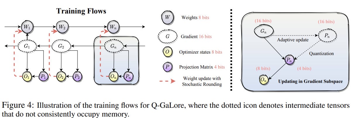
Low precision training with low-rank gradients: This method quantizes the entire model to 8-bits (INT8) and the projection matrix to 4-bits, reducing memory requirements by about 28.57%. It still uses BFloat16 precision for calculations involving activations and gradients to maintain efficiency.
Lazy layer-wise subspace exploration: This technique optimizes how often gradient spaces and projection matrices are recomputed based on the training dynamics of different layers. Some layers converge early, some stabilize within a specific window, and others keep changing. By computing the cosine similarity of projection matrices over previous intervals and adjusting the update frequency when the similarity exceeds a threshold, it reduces the need for SVD calls by over 60%. Moreover, it allows further quantization of projection matrices, cutting the memory cost of optimizer states by an additional 25%.
In every training iteration, the full-rank gradients are projected into a low-rank format using SVD based on the adaptive strategy mentioned above. To save memory, the projection matrix is quantized to 4-bits. Once the optimizer states are updated with the low-rank gradients, they are projected back to full-rank. Throughout the training, model weights are maintained in low precision (INT8) and updated using Stochastic Rounding (rounding based on probabilities, the probability being the distance to two of the nearest round value). This method captures the subtle gradient nuances, providing an unbiased estimate of the high-precision weights. Additionally, it uses fused backward operations for parameter updates as in LoMO. Calculate the gradient of a layer, update the parameters, and move on to the previous layer so that at one point, you only need to store the gradients of only one layer thus reducing memory footprint tremendously.
For pre-training, Q-GaLore reduces memory requirements by 61% and 30% compared to full-rank training and GaLore, respectively, across model sizes from 60M to 7B. Notably, Q-GaLore enables training a LLaMA-7B model on a single NVIDIA RTX 4060 Ti with 16GB of memory, achieving performance comparable to full-rank training. In fine-tuning, Q-GaLore matches the performance of state-of-the-art low-rank approaches, reducing memory consumption by up to 50% compared to LoRA and GaLore, and consistently outperforming QLoRA at the same memory cost.
Mistral AI’s Codestral and MathΣtral
Codestral Mamba is a model designed specifically for code generation. It breaks away from traditional Transformer models, which rely on attention mechanisms that scale quadratically with input sequence length. This quadratic scaling often results in inefficiencies and high resource demands for longer sequences. In contrast, Mamba models use linear time inference, making it way more efficient and theoretically able to handle sequences of infinite length. This enables Codestral Mamba to provide quick responses regardless of input size, making it highly effective for code productivity tasks.
Codestral incorporates 64 Mamba2 (paper) blocks, featuring SiLU activation and RMSNorm layers. It has a hidden size of 4096 and an intermediate size of 18560. This configuration results in a 1D convolution layer with both input and output channels set to 10240 and a kernel size of 4.
Looking at the results, this 7B model easily outperforms its counterparts, including CodeLlama 34B. It was tested on context lengths of up to 256K. While its predecessor, Codestral 22B, still holds the top spot, being a Transformer, its inference capabilities scale quadratically with input length, increasing response latency.
That's not all. Mistral also dropped MathΣtral, a model focused on mathematical reasoning and scientific discovery, in honor of Archimedes' 2311th anniversary. It is part of Mistral AI’s broader initiative to support academic projects in collaboration with Project Numina. This new model aims to assist in solving advanced mathematical problems that require complex, multi-step logical reasoning.
Let’s compare MathΣtral with the Gemma 2 9B model we discussed today. MathΣtral has a hidden size of 4096, whereas Gemma 2 9B has 3584, allowing for more information flow. Both models share the same intermediate size. MathΣtral also uses GQA, but with 32 attention heads, double the amount in Gemma 2 9B. To balance the increased hidden size and attention heads, MathΣtral has 32 hidden layers, ten fewer than Gemma 2 9B. You might think they opted for a wider network over a deeper one, but remember, MathΣtral is a 7B model, not a 9B, so it’s still a fairly deeper network.
One of the key differences is the context window. MathΣtral has a 32K context window. For comparison, DeepSeek Math and Qwen2 have context windows of 128K, while Gemma2 has only 8K. MathΣtral might have found a balance here, which could explain its superior performance. Although DeepSeek Math and Qwen2 outperform it in some cases, MathΣtral could be a better choice if you're looking for a well-rounded model for reasoning. Qwen2 is not specifically fine tuned for math so that makes it all the more commendable.
All in all, mistral.ai has been continuously releasing open models. We people don’t really need them to release mistral large or something. We can’t even run them. These < 30B models are great for enthusiasts to try. For anything larger, there’s always models hosted on the web. If you really are privacy focused and have the compute to run big models, you’re better off fine tuning whatever is available out there for your use case and using them. If that isn’t enough something like model merging can help you go a long way.


