AI Unplugged 10: KAN, xLSTM, OpenAI GPT4o and Google I/O updates, Alpha Fold 3, Fishing for MagiKarp
Insights over Information
Table of Contents:
KAN: Kolmogorov–Arnold Networks
xLSTM
Fishing for Magikarp: Untrained tokens
Alpha Fold 3
OpenAI Spring Update
Google I/O 2024
KAN: Kolmogorov–Arnold Networks
So this caught a lot of eyeballs last week on Twitter and various other ML spaces. Kolmogorov Arnold Networks or KAN in short, are an alternative (to avoid saying replacement) to MLP. Also on a completely unrelated note, read up about Kolmogorov Complexity and the paradox associated. MLPs have been the backbone of many deep neural networks. They’re after all a pseudo copy of what happens inside a human brain. Unlike ConvNets or RNNs, MLPs don’t have strong inductive biases, meaning the architecture itself isn’t biased towards some form of data or patterns. Note that an implication of this is that they need more data to learn patterns. Here’s the github repo for the same.
Every other architecture had its moments of glory and criticism but MLPs seem to have stood the test of time. Now this KAN is trying to challenge the status quo. If you remember MLP, there are layers and each layer has a few neurons. The neurons (nodes if you think of it in terms of a graph) are connected by weights (edges). Thus weighted sum is then passed into an activation function which becomes the value of that neuron in that layer. KAN tries to flip the script around. Instead of having a fixed activation at the neurons, KAN has learnable activations at each edge (where there previously was a weight). The accumulation is a summation and is done at nodes.
MLPs are backed by the Universal Approximation Theorem which states that a FFNN with single hidden layer (with sufficiently large num of neurons) can approximate any continuous function. On the other hand, KAN is backed by Kolmogorov-Arnold Representation Theorem which states that any multivariate (function on multiple variables) continuous can be represented as composition of continuous single variable functions. Do note that these aren’t the only ways to approximate functions. One can use polynomials as the basis of arbitrary degrees to approximate functions. The other option is to use sinusoidal functions as the basis, something similar to Fourier transform where we represent a function (signal) as the sum of sinusoidal. But the space you can represent with these might not be as vast as that with an FFNN.
So why look for MLP alternatives you ask? MLPs suffer from the curse of dimensionality. And they are also not very interpretable. One can dissect an attention layer to understand the connections aka what tokens attend to what tokens in a given layer. One can also visually understand what a convnet layer sees by checking activation mappings. But MLPs are pretty much pure black boxes. And once you train an MLP, you can’t even increase its expressivity by adding new neurons. That would require full training. One can add new layers but the depth of the network can only take so far. These are enough motivations to look beyond MLPs. Who knows what the world has to offer?
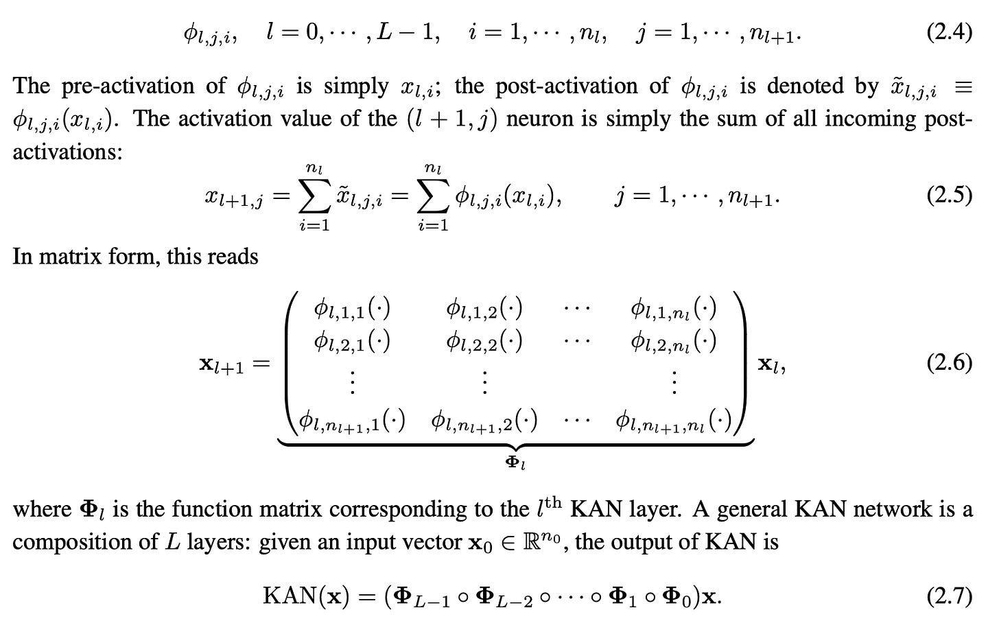
This is what the equation in Kolmogorov-Arnold representation theorem looks like. Note that in the definition, f is a smooth function from [0,1]^n → R. The equation looks like a 2 layer thing. The first layer does the inner summation resulting in 2n+1 outputs and the second layer takes all of those and returns a single number. But the thing is there is no restriction on those univariate functions. These in theory can be discontinuous or even fractal which are hard to learn. The theorem doesn’t provide a way to even calculate those functions. To circumvent this, we can extend the same to have multiple layers.
Now the key idea is to parameterize the 1D functions to some known family or type of functions. This is where the authors choose B-splines. Splines are a way to interpolate between a given set of points. Here’s a wonderful video about splines and B-splines I highly recommend you guys to watch it. Splines’ uses go from Game development to Computer Graphics and whatnot. Who knew that a random Math video with nice animations I watched few months ago would come in handy to explain an ML paper :) For those who like when I explain things, below is a brief of the same.
Given a set of points, one can create a function passing through them in multiple ways. You can just join each consecutive pair of points with line segments, like you do on normal graphs, like stock prices or growth numbers. You can also join three consecutive points with a quadratic function. And the higher the number of points considered, the higher the degree of curve. Degree 3 functions (polynomials) are used in general and there are constrains to make the function continuous at points and sometimes even differentiable. You can also choose to have a function that is double differentiable but slightly off from the points. This is a B-spline and these can be of any order (say k) Each of the methods give rise to a type of splines. You can play around here. The red curve is the spline fitting the green points.

Here you linearly interpolate between say 3 points. That gives 2 points one on each line segment. Now if you linearly interpolate on those, you get curves. And above are different ways you can represent the path traced. t is the variable that controls where along the path we are. Pi is the set of points.
The advantages of B-Splines are that they’re locally controllable. Meaning that you can change the function at/around a point without needing to change the entirity giving us finer control without drastic changes. This is how the whole math is defined. ni is the number of nodes in ith layer.
With all the setup out of the way, we can zoom into the details… We’ve been saying ϕ(x) but what is ϕ(x)? Here’s how you define it. b(x) acts like a bias and Ci’s are learnable weights.
All the theory is well and good but what about performance you ask? This is where we have to take things with a pinch of salt. They only do experiments on toy datasets.
So if you played around with splines, you’d understand that with more data points, you can control the curves better to fit your target. But each point adds more complexity in calculation. But the best part is, you can always extend later unlike MLPs. Suppose you have a grid and a corresponding spline coefficients, you create new coefficients, more in number, which minimise mean squared error between the two.
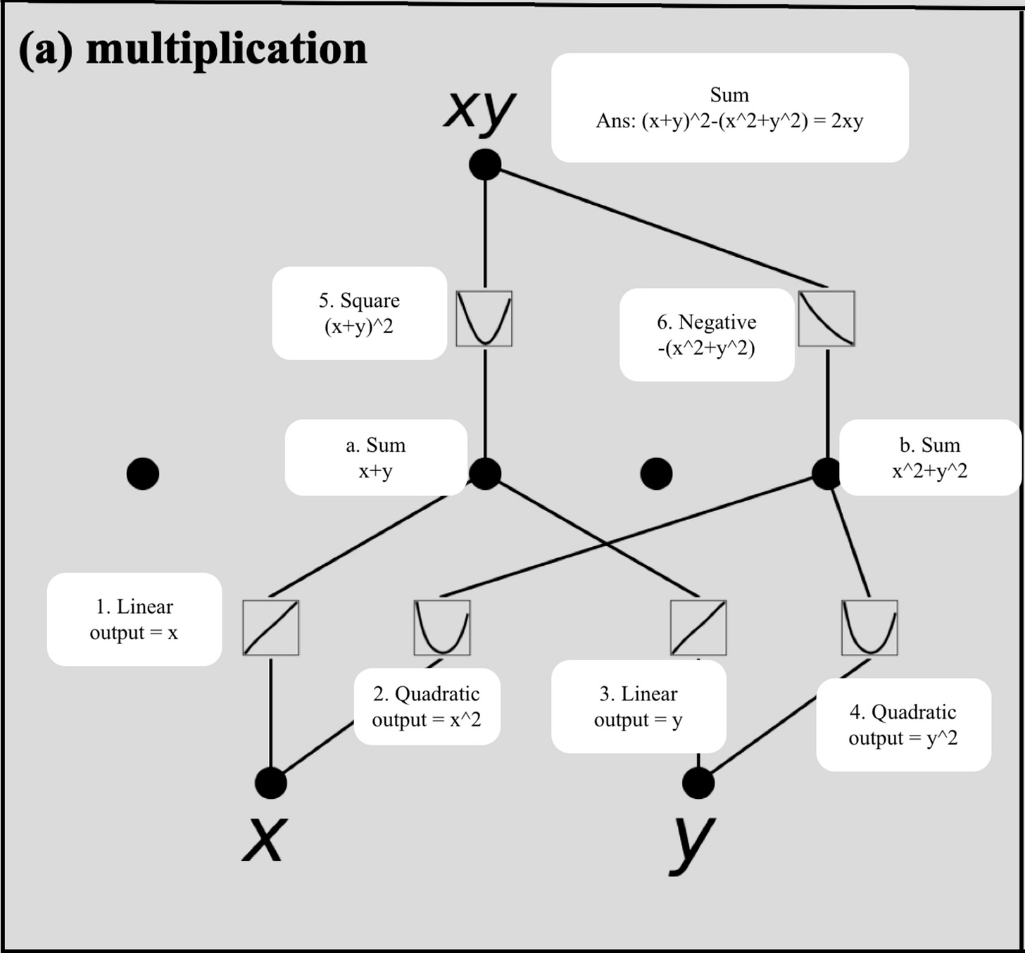
Coming to the interpretability, one can look at each of the edges and understand the activations. A node’s input is basically addition of those activations. And one can easily visualise those splines. Here’s an example of how KAN does multiplication given x and y as input. You can see the activations (splines) closely represent linear in labels 1 and 3, quadratic functions (squaring) in labels 2 and 4. At nodes (a and b), we just sum the inputs. Then at 5, we square again, while taking negative at 6. The whole is then summed up for the final answer. Note that the mismatch between xy and 2xy as labeled can be because the leading coefficient of any of the quadratic functions might be 1/2 (or anything other than 1). But you get the idea.
The authors also show that KANs don’t suffer from catastrophic forgetting (yet again, a toy example). They also provide a way to snap thus inspected activations to known functions like sines, exponentials etc etc. The worst part about KAN is the multiplication matrix (eq 2.6) is not constant across data (unlike MLP). So one has to calculate the matrix for every input separately. Thus adding to compute time. But the saving grace is, you can train KAN with much fewer parameters and outperform FFNNs.
Critical Take:
Interpretability is a big win but performance on real world scenarios unknown
Can’t take advantage of optimised matrix multiplications unfortunately
MLPs in the examples might be undertrained and KANs might be overfitting. Need science behind KANs to grow exponentially to start replacing MLPs
Being too sensitive locally can mean they might overfit to noisy samples
xLSTM: Extended Long Short-term memory
Remember LSTMs? Those that were used for Language Modelling in the pre-transformer era aka pre-2017. That was 7 years ago. Feel old yet? With all the architectures making an appearance or a comeback, for eg, RNNs with Infini-Attention ( well at least similar enough) or Based and new architectures like Mamba and Jamba, why not give LSTMs another try right… Scale was what brought LLMs the powers and scale is what other architectures lacked, until now.
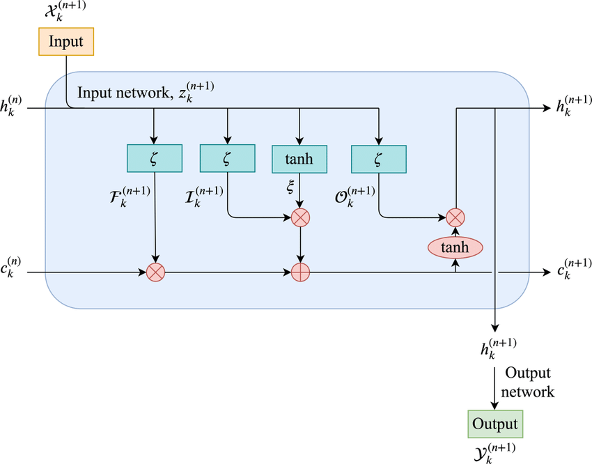
To recall LSTM, LSTM stands for Long Short-Term Memory. This was a natural successor to RNNs which had the problem of forgetting things due to limited memory. LSTMs had a mechanism to selectively remember things unlike RNNs using something called Forget Gate. Another drawback with RNNs was the issue of vanishing gradients, where the gradients kept reducing in magnitude as we went from right to left in sequence for back propagation.
To improve LSTMs, we need to know what the drawbacks of LSTMs are, at least as compared to Transformers. LSTMs have limited memory, generally a single vector which seriously limits its ability to look back. Sequential decoding constraint means that these aren’t parallelizable during training like Transformers are.
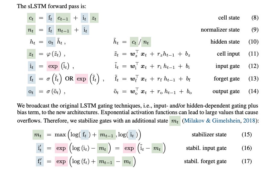
There are two parts to the whole xLSTM network. sLSTM and mLSTM to address the above drawbacks. Lets start with sLSTM. There are minor changes here. Instead of sigmoid for gating, they use exponential gating. And there is another state to stablize the whole thing.
Then comes mLSTM which basically upgrades the memory. They use something similar to transformers with Queries, Keys and Values (I Know… yet again a new architecture but relies on QKV for memory), after all, this is the most intuitive way to store and retrieve information. So the ct from now becomes a matrix.
Then there’s also residual connection. Because they are known to stablize training and generally networks are initialised around zero and it’d be easier to learn the change or delta instead of learning the entire information. And if you see above, the memory computation has precomputed VtKt just like Linear Attention or that used in Inifini-Attention. This makes it linear in sequence length (quadratic in hidden dimension but hidden dimension is fixed so thats not considered a big problem and as of now, anything with >4k or 8k context is bigger than its hidden dimension).
One thing to note from the above image is, Transformers are very very good with retrieval. Even at small model sizes, their accuracy is ~100% as they can store the information without needing to compress anything. Good thing is, xLSTM get better as model size grows. There are ablation studies for the ratios of mLSTM to sLSTM just like Jamba did for Mamba:Attention ratios.
Lastly, the most promising thing we have is sequence length extrapolation. This is one area where Transformers struggle because they tend to overfit/memorise positions and are completely broken when sequence length exceeds the training sequence lengths. In the below image, perplexity shoots up after 2048 tokens. But the other architectures like RKWV and xLSTM (both are recurrent and hence don’t need to have position index and hence no problems of memorisation) generalise very well.
Critical Take:
Yet another alternative to transformers. But Mamba is the reigning contender. Unfortunately no public model to validate claims or test performance
Training parallelisability is something I’m still unsure of. Mamba tackled this too.
Fishing for Magikarp: Finding untrained tokens
LLMs use tokenisers to know when to split a word into tokens and what a token means. There are multiple different tokenisers like Byte Pair Encoding (commonly used in llama models), TikToken (commonly used in GPT-3/4 family). Each tokeniser has a set of tokens it resolves things into called as vocabulary. But not all tokens are created equal. Some might occur more frequently than others (like english word the), some are longer than others, some have spaces prefixed etc etc. All these are determined by how one converts raw text into vocabulary.
Generally, there are iterative approaches on the text lengths depending on the frequency of the adjoined string. But due to this, we might end up with some tokens which are never returned upon tokenisation. For example, hypothetically if theres a token called new_%token (say token ID of 163) but new_ (say 225) and %token (say 1008) are tokens in themselves and the tokeniser looks splits based on special characters, we’d always end up with tokens 225 and 1008 but never have any string resulting in the 163. Hence while training, these tokens’ embeddings are left relatively untouched. So among a vocabulary of say 32K, one might find a few dozen tokens like this. If you see llama-3-8B’s vocabulary, there are even reserved tokens which are most likely under-trained/untrained.
Due to being untrained, the models wouldn’t know what to do when they see these tokens. They can behave unexpectedly, possibly randomly or maybe breaking their alignments. This paper is an attempt at finding/fishing out such tokens.
This is Cohere CmdR+ running on HuggingChat. While it was able to replicate all the other tokens correctly, it failed replicating its own “untrained” tokens aka AddLanguageSpecificText and ephritidae. Note that _coachTry is gemma’s untrained token and Cohere would not have problems replicating that. The full list can be seen here
So how does one even find or detect these kinds of tokens? One way is to look at the so called UnEmbedding matrix U which is basically the lm_head which takes logits and converts them to vectors in vocabulary space. Another key intuition is the tokens like <s> which mark beginning of sentence, which are used in training but are never predicted (cuz no text has <s> in the middle). Also one can look at L2 norm of the embeddings in case of untrained tokens as those aren’t effected by back propogation.
Max(token prob in verification) is basically trying out a few inferences and calculating each token’s prob over those inferences and finding out the max of each of those. If such max probability is in relatively high range (say >10^-2), that means the model can predict those tokens sometime or the other. The rest, where max(prob) is very small (say <10^-6), the model has never seen those tokens occur in the training data. From the above image (right half), there’s a high correlation between max prob and L2 norm of embeddings. The left half of the image is cosine distance between Unembedding (without 1st principal component) matrix and max probs. After removing the 1st PC (one can argue the same for/after removing more components), if the distance is very less that means those tokens are basically close to random or basically not contributing anything to the Unembedding or its principal components (the essence), hence untrained.
So if you ever work with LLMs, make sure that those untrained tokens are not input as part of the user’s prompt. Maybe modify the tokenizer, maybe have a hard restriction on the tokens with regex, just have guardrails to not fall into these pits.
OpenAI: GPT4o
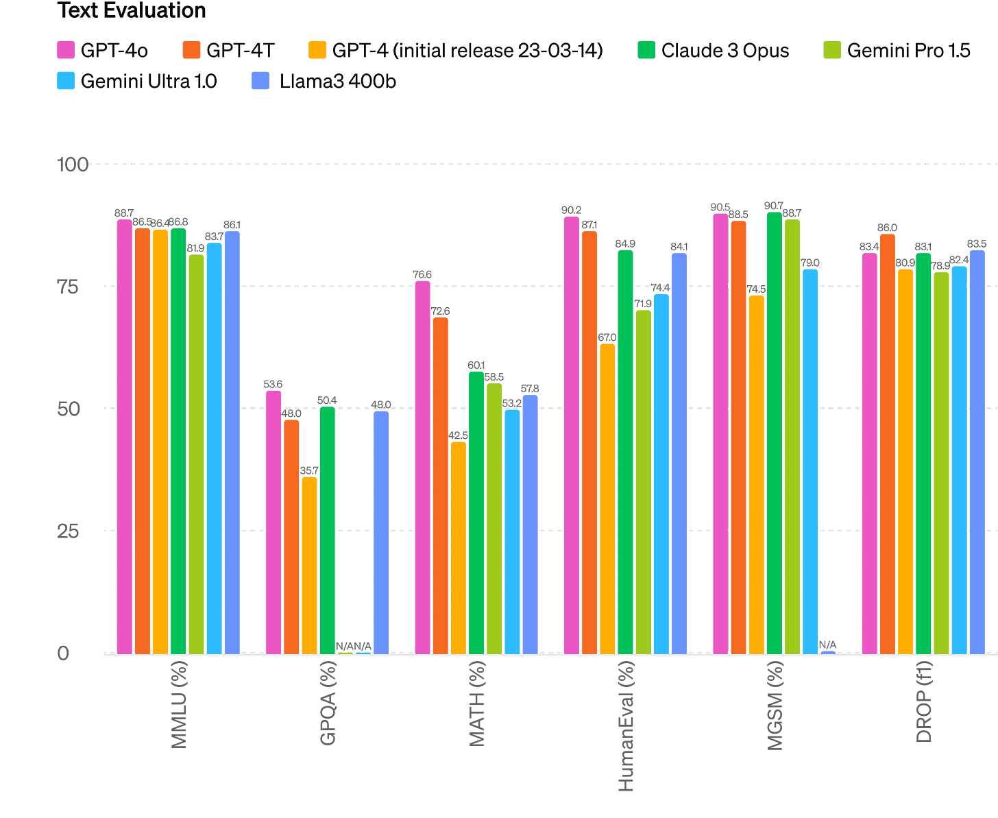
The new addition to the GPT family of models. o stands for Omni (meaning all modalities). This is a natively multimodal model which means no more of converting audio into text or text to audio. The model inherently understands audio/images. The model is blazingly fast. I think there’s Quantisation and Speculative decoding going on behind the scenes. It outperforms GPT4-Turbo on various benchmarks and it is free to use via ChatGPT (hoorah!).
It uses a new tokeniser, which improves on a lot of Non-English languages. Shrinking the tokens used by factors of 2-5x. Combine this with already fast model, that is a good 5-10x speedup.
There’s also a MacOS App (unfortunately I don’t yet have access to) that can access your screen (no more screenshotting) and help you. Maybe this is one way openAI gets our training data, who knows. There’s no Windows app (yet). Maybe Microsoft would integrate something similar, brand it as Copilot 2.0 in rumoured Windows 12?
This is the same model that has been going around by the name gpt-chatbot on LMSys leaderboard. But people have been seeing some weird issues (like typos) with the model so be a little careful before replacing your current Go-To.
I asked it our usual Pound of bricks vs Kilo of feathers question. It succeeded unlike GPT3. Even on my trial to put it off, it doesn’t budge. It falters in the Yann Le Cunn’s 7 gear problem though.
Google I/O 2024: Gemini Era
Gemini 1.5 Flash, smaller and hence faster than Gemini 1.5 Pro
Gemini 1.5Pro get 2M context window.
Imagen3 launched.
Veo, a text to video model. 1080p generations
TPU v6 Trillum, 4.7x faster than v5.
Video as context for Google Search (think google lens but video)
Gems, basically GPTs for Gemini
Gemma2 27B to launch in June :)
We’ll definitely look into these in the upcoming days. Its already a little long for today. Gemini on Google AI Studio does pass our bricks vs feathers question. Maybe we’re slowly moving away from over alignment looking at how the models are progressing over time. GPT-3.5 on ChatGPT and Gemini 1 failed at the same previously.
Google’s biggest super power is Search and Google Account. We use it everyday, especially on Android. So it has a lot of personal information for its context and has the ability to be the most helpful assistant if done right.
Alpha Fold 3
Alpha Fold 3 is the 3rd generation in Alpha Fold series of models by Google Deepmind published in Nature. The models are trained on Protein structures and hence learn how they interact, bond etc. Going one step beyond, this generation of models are not just restricted to proteins being able to model more biomolecules. Alpha is a common prefix Deepmind uses for their models. Alpha-Go for the game Go, AlphaZero for Chess for example.
There’s also AlphaFold Server where you can interact with the model. I’m not an expert in Biology so excuse me for not playing around :)


